The Bias in Line Betting Revisited

Some blogs almost write themselves. This hasn't been one of them.

It all started when I read a journal article - to which I'd now link if I could find the darned thing again - that suggested a bias in NFL (or maybe it was College Football) spread betting markets arising from bookmakers' tendency to over-correct when a team won on line betting. The authors found that after a team won on line betting one week it was less likely to win on line betting next week because it was forced to overcome too large a handicap.

Naturally, I wondered if this was also true of AFL spread betting.

What Makes a Team's Start Vary from Week-to-Week?

In the process of investigating that question, I wound up wondering about the process of setting handicaps in the first place and what causes a team's handicap to change from one week to the next.

Logically, I reckoned, the start that a team receives could be described by this equation:

Start received by Team A (playing Team B) = (Quality of Team B - Quality of Team A) - Home Status for Team A

In words, the start that a team gets is a function of its quality relative to its opponent's (measured in points) and whether or not it's playing at home. The stronger a team's opponent the larger will be the start, and there'll be a deduction if the team's playing at home. This formulation of start assumes that game venue only ever has a positive effect on one team and not an additional, negative effect on the other. It excludes the possibility that a side might be a P point worse side whenever it plays away from home.

With that as the equation for the start that a team receives, the change in that start from one week to the next can be written as:

Change in Start received by Team A = Change in Quality of Team A + Difference in Quality of Teams played in successive weeks + Change in Home Status for Team A

To use this equation for we need to come up with proxies for as many of the terms that we can. Firstly then, what might a bookie use to reassess the quality of a particular team? An obvious choice is the performance of that team in the previous week relative to the bookie's expectations - which is exactly what the handicap adjusted margin for the previous week measures.

Next, we could define the change in home status as follows:

• Change in home status = +1 if a team is playing at home this week and played away or at a neutral venue in the previous week
• Change in home status = -1 if a team is playing away or at a neutral venue this week and played at home in the previous week
• Change in home status = 0 otherwise

This formulation implies that there's no difference between playing away and playing at a neutral venue. Varying this assumption is something that I might explore in a future blog.

From Theory to Practicality: Fitting a Model

(well, actually there's a bit more theory too ...)

Having identified a way to quantify the change in a team's quality and the change in its home status we can now run a linear regression in which, for simplicity, I've further assumed that home ground advantage is the same for every team.

We get the following result using all home-and-away data for seasons 2006 to 2010:

For a team (designated to be) playing at home in the current week:

Change in start = -2.453 - 0.072 x HAM in Previous Week - 8.241 x Change in Home Status

For a team (designated to be) playing away in the current week:

Change in start = 3.035 - 0.155 x HAM in Previous Week - 8.241 x Change in Home Status

These equations explain about 15.7% of the variability in the change in start and all of the coefficients (except the intercept) are statistically significant at the 1% level or higher.

(You might notice that I've not included any variable to capture the change in opponent quality. Doubtless that variable would explain a significant proportion of the otherwise unexplained variability in change in start but it suffers from the incurable defect of being unmeasurable for previous and for future games. That renders it not especially useful for model fitting or for forecasting purposes.

Whilst that's a shame from the point of view of better modelling the change in teams' start from week-to-week, the good news is that leaving this variable out almost certainly doesn't distort the coefficients for the variables that we have included. Technically, the potential problem we have in leaving out a measure of the change in opponent quality is what's called an omitted variable bias, but such bias disappears if the the variables we have included are uncorrelated with the one we've omitted. I think we can make a reasonable case that the difference in the quality of successive opponents is unlikely to be correlated with a team's HAM in the previous week, and is also unlikely to be correlated with the change in a team's home status.)

Using these equations and historical home status and HAM data, we can calculate that the average (designated) home team receives 8 fewer points start than it did in the previous week, and the average (designated) away team receives 8 points more.

All of which Means Exactly What Now?

Okay, so what do these equations tell us?

Firstly let's consider teams playing at home in the current week. The nature of the AFL draw is such that it's more likely than not that a team playing at home in one week played away in the previous week in which case the Change in Home Status for that team will be +1 and their equation can be rewritten as

Change in Start = -10.694 - 0.072 x HAM in Previous Week

So, the start for a home team will tend to drop by about 10.7 points relative to the start it received in the previous week (because they're at home this week) plus about another 1 point for every 14.5 points lower their HAM was in the previous week. Remember: the more positive the HAM, the larger the margin by which the spread was covered.

Next, let's look at teams playing away in the current week. For them it's more likely than not that they played at home in the previous week in which case the Change in Home Status will be -1 for them and their equation can be rewritten as

Change in Start = 11.276 - 0.155 x HAM in Previous Week

Their start, therefore, will tend to increase by about 11.3 points relative to the previous week (because they're away this week) less 1 point for every 6.5 points lower their HAM was in the previous week.

Away teams, therefore, are penalised more heavily for larger HAMs than are home teams.

This I offer as one source of potential bias, similar to the bias that was found in the original article I read.

Proving the Bias

As a simple way of quantifying any bias I've fitted what's called a binary logit to estimate the following model:

Probability of Winning on Line Betting = f(Result on Line Betting in Previous Week, Start Received, Home Team Status)

This model will detect any bias in line betting results that's due to an over-reaction to the previous week's line betting results, a tendency for teams receiving particular sized starts to win or lose too often, or to a team's home team status.

The result is as follows:

logit(Probability of Winning on Line Betting) = -0.0269 + 0.054 x Previous Line Result + 0.001 x Start Received + 0.124 x Home Team Status

The only coefficient that's statistically significant in that equation is the one on Home Team Status and it's significant at the 5% level. This coefficient is positive, which implies that home teams win on line betting more often than they should.

Using this equation we can quantify how much more often. An away team, we find, has about a 46% probability of winning on line betting, a team playing at a neutral venue has about a 49% probability, and a team playing at home has about a 52% probability.

That is undoubtedly a bias, but I have two pieces of bad news about it. Firstly, it's not large enough to overcome the vig on line betting at $1.90 and secondly, it disappeared in 2010.

Do Margins Behave Like Starts?

We now know something about how the points start given by the TAB Sportsbet bookie responds to a team's change in estimated quality and to a change in a team's home status. Do the actual game margins respond similarly?

One way to find this out is to use exactly the same equation as we used above, replacing Change in Start with Change in Margin and defining the change in a team's margin as its margin of victory this week less its margin of victory last week (where victory margins are negative for losses).

If we do that and run the new regression model, we get the following:

For a team (designated to be) playing at home in the current week:

Change in Margin = 4.058 - 0.865 x HAM in Previous Week + 8.801 x Change in Home Status

For a team (designated to be) playing away in the current week:

Change in Margin = -4.571 - 0.865 x HAM in Previous Week + 8.801 x Change in Home Status

These equations explain an impressive 38.7% of the variability in the change in margin. We can simplify them, as we did for the regression equations for Change in Start, by using the fact that the draw tends to alternate team's home and away status from one week to the next.

So, for home teams:

Change in Margin = 12.859 - 0.865 x HAM in Previous Week

While, for away teams:

Change in Margin = -13.372 - 0.865 x HAM in Previous Week

At first blush it seems a little surprising that a team's HAM in the previous week is negatively correlated with its change in margin. Why should that be the case?

It's a phenomenon that we've discussed before: regression to the mean. What these equations are saying are that teams that perform better than expected in one week - where expectation is measured relative to the line betting handicap - are likely to win by slightly less than they did in the previous week or lose by slightly more.

What's particularly interesting is that home teams and away teams show mean regression to the same degree. The TAB Sportsbet bookie, however, hasn't always behaved as if this was the case.

Another Approach to the Source of the Bias

Bringing the Change in Start and Change in Margin equations together provides another window into the home team bias.

The simplified equations for Change in Start were:

Home Teams: Change in Start = -10.694 - 0.072 x HAM in Previous Week

Away Teams: Change in Start = 11.276 - 0.155 x HAM in Previous Week

So, for teams whose previous HAM was around zero (which is what the average HAM should be), the typical change in start will be around 11 points - a reduction for home teams, and an increase for away teams.

The simplified equations for Change in Margin were:

Home Teams: Change in Margin = 12.859 - 0.865 x HAM in Previous Week

Away Teams: Change in Margin = -13.372 - 0.865 x HAM in Previous Week

So, for teams whose previous HAM was around zero, the typical change in margin will be around 13 points - an increase for home teams, and a decrease for away teams.

Overall the 11-point v 13-point disparity favours home teams since they enjoy the larger margin increase relative to the smaller decrease in start, and it disfavours away teams since they suffer a larger margin decrease relative to the smaller increase in start.

To Conclude

Historically, home teams win on line betting more often than away teams. That means home teams tend to receive too much start and away teams too little.

I've offered two possible reasons for this:

1. Away teams suffer larger reductions in their handicaps for a given previous weeks' HAM
2. For teams with near-zero previous week HAMs, starts only adjust by about 11 points when a team's home status changes but margins change by about 13 points. This favours home teams because the increase in their expected margin exceeds the expected decrease in their start, and works against away teams for the opposite reason.

If you've made it this far, my sincere thanks. I reckon your brain's earned a spell; mine certainly has.

Adding Some Spline to Your Models

Creating the recent blog on predicting the Grand Final margin based on the difference in the teams' MARS Ratings set me off once again down the path of building simple models to predict game margin.

It usually doesn't take much.

Firstly, here's a simple linear model using MARS Ratings differences that repeats what I did for that recent blog post but uses every game since 1999, not just Grand Finals.

It suggests that you can predict game margins - from the viewpoint of the home team - by completing the following steps:

1. subtract the away team's MARS Rating from the home team's MARS Rating
2. multiply this difference by 0.736
3. add 9.871 to the result you get in 2.

One interesting feature of this model is that it suggests that home ground advantage is worth about 10 points.

The R-squared number that appears on the chart tells you that this model explains 21.1% of the variability is game margins.

You might recall we've found previously that we can do better than this by using the home team's victory probability implied by its head-to-head price.

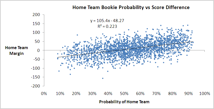
This model says that you can predict the home team margin by multiplying its implicit probability by 105.4 and then subtracting 48.27. It explains 22.3% of the observed variability in game margins, or a little over 1% more than we can explain with the simple model based on MARS Ratings.

With this model we can obtain another estimate of the home team advantage by forecasting the margin with a home team probability of 50%. That gives an estimate of 4.4 points, which is much smaller than we obtained with the MARS-based model earlier.

(EDIT: On reflection, I should have been clearer about the relative interpretation of this estimate of home ground advantage in comparison to that from the MARS Rating based model above. They're not measuring the same thing.

The earlier estimate of about 10 points is a more natural estimate of home ground advantage. It's an estimate of how many more points a home team can be expected to score than an away team of equal quality based on MARS Rating, since the MARS Rating of a team for a particular game does not include any allowance for whether or not it's playing at home or away.

In comparison, this latest estimate of 4.4 points is a measure of the "unexpected" home ground advantage that has historically accrued to home teams, over-and-above the advantage that's already built into the bookie's probabilities. It's a measure of how many more points home teams have scored than away teams when the bookie has rated both teams as even money chances, taking into account the fact that one of the teams is (possibly) at home.

It's entirely possible that the true home ground advantage is about 10 points and that, historically, the bookie has priced only about 5 or 6 points into the head-to-head prices, leaving the excess of 4.4 that we're seeing. In fact, this is, if memory serves me, consistent with earlier analyses that suggested home teams have been receiving an unwarranted benefit of about 2 points per game on line betting.

Which, again, is why MAFL wagers on home teams.)

Perhaps we can transform the probability variable and explain even more of the variability in game margins.

In another earlier blog we found that the handicap a team received could be explained by using what's called the logit transformation of the bookie's probability, which is ln(Prob/(1-Prob)).

Let's try that.

We do see some improvement in the fit, but it's only another 0.2% to 22.5%. Once again we can estimate home ground advantage by evaluating this model with a probability of 50%. That gives us 4.4 points, the same as we obtained with the previous bookie-probability based model.

A quick model-fitting analysis of the data in Eureqa gives us one more transformation to try: exp(Prob). Here's how that works out:

We explain another 0.1% of the variability with this model as we inch our way to 22.6%. With this model the estimated home-ground advantage is 2.6 points, which is the lowest we've seen so far.

If you look closely at the first model we built using bookie probabilities you'll notice that there seems to be more points above the fitted line than below it for probabilities from somewhere around 60% onwards.

Statistically, there are various ways that we could deal with this, one of which is by using Multivariate Adaptive Regression Splines.

(The algorithm in R - the statistical package that I use for most of my analysis - with which I created my MARS models is called earth since, for legal reasons, it can't be called MARS. There is, however, another R package that also creates MARS models, albeit in a different format. The maintainer of the earth package couldn't resist the temptation not to call the function that converts from one model format to the other mars.to.earth. Nice.)

The benefit that MARS models bring us is the ability to incorporate 'kinks' in the model and to let the data determine how many such kinks to incorporate and where to place them.

Running earth on the bookie probability and margin data gives the following model:

Predicted Margin = 20.7799 + if(Prob > 0.6898155, 162.37738 x (Prob - 0.6898155),0) + if(Prob < 0.6898155, -91.86478 x (0.6898155 - Prob),0)

This is a model with one kink at a probability of around 69%, and it does a slightly better job at explaining the variability in game margins: it gives us an R-squared of 22.7%.

When you overlay it on the actual data, it looks like this.

You can see the model's distinctive kink in the diagram, by virtue of which it seems to do a better job of dissecting the data for games with higher probabilities.

It's hard to keep all of these models based on bookie probability in our head, so let's bring them together by charting their predictions for a range of bookie probabilities.

For probabilities between about 30% and 70%, which approximately equates to prices in the $1.35 to $3.15 range, all four models give roughly the same margin prediction for a given bookie probability. They differ, however, outside that range of probabilities, by up to 10-15 points. Since only about 37% of games have bookie probabilities in this range, none of the models is penalised too heavily for producing errant margin forecasts for these probability values.

So far then, the best model we've produced has used only bookie probability and a MARS modelling approach.

Let's finish by adding the other MARS back into the equation - my MARS Ratings, which bear no resemblance to the MARS algorithm, and just happen to share a name. A bit like John Howard and John Howard.

This gives us the following model:

Predicted Margin = 14.487934 + if(Prob > 0.6898155, 78.090701 x (Prob - 0.6898155),0) + if(Prob < 0.6898155, -75.579198 x (0.6898155 - Prob),0) + if(MARS_Diff < -7.29, 0, 0.399591 x (MARS_Diff + 7.29)

The model described by this equation is kinked with respect to bookie probability in much the same way as the previous model. There's a single kink located at the same probability, though the slope to the left and right of the kink is smaller in this latest model.

There's also a kink for the MARS Rating variable (which I've called MARS_Diff here), but it's a kink of a different kind. For MARS Ratings differences below -7.29 Ratings points - that is, where the home team is rated 7.29 Ratings points or more below the away team - the contribution of the Ratings difference to the predicted margin is 0. Then, for every 1 Rating point increase in the difference above -7.29, the predicted margin goes up by about 0.4 points.

This final model, which I think can still legitimately be called a simple one, has an R-squared of 23.5%. That's a further increase of 0.8%, which can loosely be thought of as the contribution of MARS Ratings to the explanation of game margins over and above that which can be explained by the bookie's probability assessment of the home team's chances.