Another Look at Forecasting Game Outcomes In-Running

Modelling the outcome of an AFL game in-running has been a recurring theme for MAFL Online.

There's this post from 2010, in which I built a single model - based on Brownian motion - that took as inputs only the game result, the Home team's lead and the time remaining at the quarter-breaks in every game. Then there's this followup post from the same year, which looked at methods for projecting the game outcome in-running, including a couple that optimally combined, post hoc, the predictions of the Brownian motion inspired model with the Bookmaker's pre-game assessment.

More recently, in this 2011 post I created a series of models, one for each quarter-break, that took a more statistical approach to combining the Bookmaker's pre-game probability assessments with the Home team's lead at a particular break.

In this blog I'm going to update and expand on the models from that 2011 post using data from seasons 2006 to 2012, in particular by investigating: 

• the best way to express the Bookmaker's pre-game assessments in the models (to date I've always used the Home team's Implicit Probability)
• the modelling benefits, if any, of including the Home team leads as at the end of all quarters in the game so far, not just at the end of the quarter for which the model is being constructed
• how knowledge of the Bookmaker's pre-game assessment of the teams diminishes, relative to knowledge about the scores at every change, as the game progresses
• how the importance of lead-size has varied from season to season

Incorporating the Bookmaker's Pre-Game Assessments

For any game I've just two pieces of information about the TAB Bookmaker's relative assessments of the competing teams: the price he's offering for the Home team, and the price he's offering for the Away team.

Actually, I don't even have two independent pieces of information if I assume that the Bookmaker's overround is constant since, given one team's price and the value of the fixed overround, the other team's price is a given.

Nonetheless, these two prices, which I'll denote H for the Home team's price, and A for the Away team's, can be combined in a variety of plausible ways to create a measure of the Home team's pre-game relative chances of victory according to the Bookmaker: 

• Home Team Implicit Probability = A / (H+A)
• Home Team Odds Ratio = (H - 1) / (A - 1)
• Home Team Inverse Odds Ratio = (A - 1) / (H - 1)
• Home Team Log Odds Ratio = log[(H-1)/(A-1)]
• Home Team Price Ratio = H / A
• Home Team Inverse Price Ratio = A / H
• Square Root Home Team Price Ratio = sqrt(H / A)
• Inverse Square Root Home Team Price Ratio = sqrt(A / H)

Any of these measures might sensibly be used for statistical modelling purposes as they're all monotonically increasing (or decreasing) with respect to the Home team price. We can also, of course, choose to include both prices, H and A, in our models. The question is then: which formulation is best?

To determine this empirically I constructed four sets of binary logit models using the data from seasons 2006 to 2012. Each set of models was constructed for use at a different point in the game: one set for use at the start of the game, another for use at Quarter time, another at Half time, and another at Three-Quarter time. Within a set of models the only thing that varied was which of the formulation of the Bookmaker's prices I used. For all models in each set the Home team result was the target variable (drawn games were ignored), and Home team leads at the end of all relevant quarters were included as regressors. 

Put another way, I created: 

• one set of models based on the score at the start of the game (ie 0-0) of the form:
  • logit(Prob(Home Team win)) = a + b x Bookmaker Price Formulation
  • another set of models based on the score at Quarter time of the form:
    • logit(Prob(Home Team win)) = a + b x Bookmaker Price Formulation + c x Home Team lead at end Q1
    • another set of models based on the score at Quarter time and Half time of the form:
      • logit(Prob(Home Team win)) = a + b x Bookmaker Price Formulation + c x Home Team lead at end Q1 + d x Home Team lead at end Q2
      • another set of models based on the score at Quarter time, Half time and Three-Quarter time of the form:
        • logit(Prob(Home Team win)) = a + b x Bookmaker Price Formulation + c x Home Team lead at end Q1 + d x Home Team lead at end Q2 + e x Home Team lead at end Q3

The best Bookmaker Price Formulation within any of the four sets of models is the one that produces the model with the lowest AIC. 

As complicated as that all probably sounds, the conclusion could not have been more straightforward: based on the AIC metric the best model within each set was the one that used the Log Odds Ratio formulation of the Bookmaker prices. For three of the four sets of models the next best formulation was to use the Home and the Away prices separately, the exception being for the models built for use at Three-Quarter time, for which our usual Home Team Implicit Probability proved superior.

Apart from its strong showing in that set, however, Home Team Implicit Probability - my unthinking go-to formulation for incorporating Bookmaker prices in models in past blogs - was generally only a mediocre performer. It finished only 3rd- or 4th-best in all other model sets. The Inverse Square Root formulation performed about equally as well, finishing 3rd in three sets and 4th in the other.

In light of the strong performance of the Log Odds Ratio it's especially interesting to note the poor performances of the Odds Ratio and Inverse Odds Ratio, which come last and second-last in all model sets. What hurts these formulations, I suspect, is how non-linearly they respond for overwhelming favourites and underdogs, which results in their values ranging from 0.0005 to 2,000 across the entire expanse of games. The log part of the Log Odds Ratio mitigates this behaviour.

To give you a sense of how the Log Odds Ratio works, here's a graph of the relationship between the Home Team Implicit Probability and the Home Team Log Odds Ratio (assuming a 105% overround).

Note how the relationship between Implicit Probability and Log Odds is virtually linear for Implicit Probabilities in the 20% to 80% range. 

There appear to be inflexion points near those probability values, beyond which the relationship becomes less linear and steeper. Since it's relatively rare to see games with Implicit Probabilities much beyond 95% (or below 5%), we don't get into the range where the Log Odds Ratio begins to asymptote most dramatically.

This non-linear behaviour might be one reason that the Log Odds Ratio formulation outperforms the Implicit Probability formulation. If the TAB Bookmaker feels constrained from shortening teams' prices too much, than a Home team price that seems to reflect an implicit probability of 90% might be based on an underlying assessment that the true probability is 95%. The Log Odds Ratio adjusts and accounts for this behaviour by providing a value that is higher than would be obtained based on a straight-line extrapolation of values for smaller implicit probabilities.

Including the Home Team Leads at the End of Each Quarter

In previous blogs, when I've constructed a model to be used at, say, Half time, I've included only the Home team's lead at Half time, ignoring the state of the game at Quarter time on the assumption that it would be largely irrelevant. Similarly, the models I've built for use at Three-Quarter time have incorporated only the Home team lead at Three-Quarter time and not its leads at Quarter time and Half time, again on the basis that these would add little if any predictive power to the model. 

Recent analyses I've done while investigating the phenomenon of momentum made me reconsider this assumption. And, it turns out, there is information content in the Home team's lead at earlier changes. 

On the left is the model for use at Quarter time. It suggests that the Home team victory probability is best described by the formula:

logit(Prob(Home Team Wins)) = 0.08 + 0.42 x Home Team Log Odds Ratio + 0.05 x Home Team Lead at End of Q1

The three asterisks in the column headed "Sig" signifies that the coefficients on the two regressors in the model are significant at the 0.1% level, while the percentages in the column headed "Imp" are estimates of the relative importance of the regressor variables in explaining variability in the target variable, here the (transformed) probability of a Home team victory. These importance values were estimated using the hier.part package in R and suggest that, at Quarter time, the variability of the ultimate victory chances of the Home team can be explained roughly in equal parts by the extent of the Home team's pre-game favouritism as expressed in the Log Odds Ratio, and the extent of the Home team's lead at Quarter time.

Moving to the next block of data we find the equivalent outputs for the model designed for use at Half time. Here we can see: 

• a significant decline in the relative importance of the Bookmaker's pre-game assessment of the Home team's chances: the relative importance of this variable falls to just 23%
• that an increase in the Home team's score (and hence lead) by one additional point at Half time has a relatively large effect on the Home team's victory probability. One way of quantifying that is to note that a Home team that started the game as equal favourite and that leads by just 12 points at Half time has the same estimated probability of victory as a Home team leads by 6 points at Half time that started as a $1.40 favourite. 
• the information content inherent in the Home team's Quarter time lead. The relevant coefficient is statistically significant, though small and, interestingly, negative, meaning that the Home team's chances at Half time are better if it trailed at Quarter time than if it led at that point. This variable's importance is assessed at about 16%.

On that last point, do bear in mind that the correlation between the Home team's Quarter time lead and its Half time lead is +0.76, so it's relatively rare for the Home team to face a sizeable deficit at Quarter time and enjoy a lead at the Half time break, and that it is the Home team's Half time lead that is far more important. 

In fact, the correlation between Home team leads for any pair of changes is quite high, as depicted in the contour plots shown at left. In these plots, the higher the correlation, the thinner and more elongated will be the contour plot.

As you'd expect, the correlations are highest for the leads at successive quarters - see the plots at positions (1,1), (2,2) and (3,2) - but even the correlation between Home team leads at the end of Q1 and the end of the game is +0.59.

From a practical point of view this means that, when we're using these models for scenario analyses, we should be cautious about setting the Home team lead at the end of a given quarter without bearing in mind the Home team lead at the end of earlier quarters.

The value of including the Home team's lead at Quarter time in this model is evidenced by the statistical significance of the coefficient on that variable. This is supported by the fact that the AIC of the model that includes this variable is lower than the AIC of the model that does not.

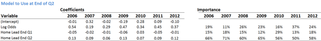
Finally, the rightmost block of data is the outputs for the model designed to be used at Three-Quarter time, and here we find: 

• a further decline in the relative importance of the Bookmaker's pre-game assessment of the Home team's chances. It now contributes only 12% to explaining the variability in the final result.
• non-trivial contributions to predicting the final outcome based on knowledge of the Home team's Quarter time and Half time leads. Together they contribute to over one-third of the explained variability. The negative coefficient on the Quarter time lead persists, but remains small yet defiantly statistically significant. Again though note that the correlation between the Home team's Quarter time lead and its Three-Quarter time lead is +0.66, and between its Half time lead and its Three-Quarter time lead is +0.87. (Again also the AIC of the model that includes these variables is smaller than the AIC of the model that does not.)
• the Home team lead at Three-Quarter time is responsible for over one-half of the explained variability in the final outcome for the Home team. The coefficient on this variable is the highest of any similar coefficients in any of the models, suggesting that a single point of lead at Three Quarter time is more important at that change than at any other.

Variable Importance Year-by-Year 

I recall claiming in other blogs that leads at particular quarter changes have been more or less important for the fates of Home teams in this year than in that year. By applying the same modelling approach that I've just described to the results for individual seasons we can see whether that claim is justified and, if so, how to quantify it.

Let's start by fitting models to the Quarter time results for each of the seasons 2006 to 2012.

On the left are the estimated coefficients, on the right the estimated variable importances.

Relatively speaking, Home team leads at Quarter time were least important in seasons 2008, 2009 and 2011, which were years in which the coefficients on the Home team Q1 lead variable were smallest and when the assessed importance of this variable was only between about 25% and 40%. 

The story for the Home team Log Odds Ratio, being the only other regressor, is a mirror image. Knowledge of the Bookmaker's pre-game prices was most relevant at Quarter time in season 2011 when it accounted for 75% of the explained variability in Home team chances, and least relevant in 2010 when it accounted for just 28%.

There are no obvious chronological trends in either the coefficients or the relative importance measures.

Next, consider models based on the Half time scores:

First, solely from the viewpoint of the Home team's victory chances, each point of Half time lead has been most important in seasons 2006, 2009 and 2012, and least important in 2008 and 2010. In terms of explaining variability in Home team outcomes, however, knowledge of the Home team's lead was most valuable in season 2007 when it accounted for 71% of the explained variability in these outcomes.

Knowledge of the Bookmaker's pre-game prices was most valuable in 2011 when it accounted for 37% of the explained variability in Home team results predicted at Half time, and least important in 2007 when it explained only 11%.

In passing I'd note that the coefficient on the Home team's Quarter time lead is negative in six of the seven seasons. Home teams really do, it seems, fare better when they trail at Quarter time - provided they go on to lead at Half (and, as we'll see, Three-Quarter) time.

Again there are no obvious trends across time in the coefficients or importance percentages.

Finally, the results based on models fitted to Three-Quarter time scores:

We find now that knowledge of the Home team's pre-game Bookmaker prices contributes only about 5% to 20% of our ability to predict the final outcome at Three-Quarter time. Knowledge of the Quarter time and Half time scores adds about another 30% to 40%, while knowledge of the Three-Quarter time scores contributes between about 45% and 65% .

Once more there's no compelling evidence for trends in the coefficient values or the importance percentages.

Summary

What we've found in this blog is that: 

• the best way to use Bookmaker pre-game prices for modelling in-running probabilities is to form a Log Odds Ratio from the two prices
• knowledge of the Home team's lead at earlier changes is, statistically speaking, valuable when projecting the final result at a subsequent change
• knowledge of the teams' pre-game prices becomes significantly less valuable in predicting a game's outcome in running as the game progresses. Roughly speaking, in percentage terms, its value halves at the end of each quarter, starting at 100%, dropping to about 50% by Quarter time, 25% by Half time, and 13% by Three-Quarter time.
• the most valuable piece of information at any quarter break is the Home team's lead at that point (though at quarter time, knowledge of the pre-game Bookmaker prices is about equally as valuable)
• the relative value of knowledge of Home team leads at each change and the pre-game Bookmaker prices has varied somewhat from season to season, though the variability in these variables' information content (measured by variable importance) has been most marked for projecting the final result at Quarter time. Variable importances for the models used to project at Half time and at Three-Quarter time have been far less volatile from season-to-season.

In the next blog we'll assess how useful the overall models might be in practice by running some scenarios using them and analysing the resulting forecasts and, most importantly, the level of statistical uncertainty associated with them.