Predicting the Final Ladder
/Discussions about the final finishing order of the 18 AFL teams are popular at the moment. In the past few weeks alone I've had an e-mail request for my latest prediction of the final ordering (which I don't have), a request to make regular updates during the season, a link to my earlier post on the teams' 2015 schedule strength turning up in a thread on the bigfooty site about the whole who-finishes-where debate, and a Twitter conversation about just how difficult it is, probabilistically speaking, to assign the correct ladder position to all 18 teams.
Read MoreWhy AFL Handicap-Adjusted Margins Are Normal : Part II
/In the previous blog on this topic I posited that the Scoring Shot production of a team could be modelled as a Poisson random variable with some predetermined mean, and that the conversion of these Scoring Shots into Goals could be modelled as a BetaBinomial with fixed conversion probability and theta (a spread parameter).
Read MoreWhy AFL Handicap-Adjusted Game Margins Are Normal
/This week, thanks to Amazon, who replaced my unreadable Kindle copy of David W Miller's Fitting Frequency Distributions: Philosophy and Practice with a dead-tree version that could easily be used as a weapon such is its heft (and assuming you had the strength to wield it), I've been reminded of the importance of motivating my distributional choices with a plausible narrative. It's not good enough, he contends, to find that, say, a Gamma Distribution fits your data set really well, you should be able to explain why it's an appropriate choice from first principles.
Read MoreThe 2014 Seasons We Might Have Had
/Each week the TAB Bookmaker forms opinions about the likely outcome of upcoming AFL matches and conveys those opinions to bettors in the form of market prices. If we assume that these opinions are unbiased reflections of the true likely outcomes, how might the competition ladder have differed from what we have now?
Read MoreModelling Team Scores as Weibull Distributions
/A recent paper on arxiv provided a statistical motivation for that interpretation of the Pythagorean Expectation formula by showing that it can be derived if we consider the two teams' scores in a contest to be distributed as independent Weibull variables under certain assumptions.
Read MoreIs That a Good Probability Score - the Brier Score Edition
/In recent blogs about the Very Simple Ratings System (VSRS) I've been using as my Probability Score metric the Brier Score, which assigns scores to probability estimates on the following basis:
Brier Score = (Actual Result - Probability Assigned to Actual Result)^2
For the purposes of calculating this score the Actual Result is treated as (0,1) variable, taking on a value of 1 if the team in question wins, and a value of zero if that team, instead, loses. Lower values of the Brier Score, which can be achieved by attaching large probabilities to teams that win or, equivalently, small probabilities to teams that lose, reflect better probability estimates.
Elsewhere in MAFL I've most commonly used, rather than the Brier Score, a variant of the Log Probability Score (LPS) in which a probability assessment is scored using the following equation:
Log Probability Score = 1 + logbase2(Probability Associated with Winning team)
In contrast with the Brier Score, higher log probabilities are associated with better probability estimates.
Both the Brier Score and the Log Probability Score metrics are what are called Proper Scoring Rules, and my preference for the LPS has been largely a matter of taste rather than of empirical evidence of superior efficacy.
Because the LPS has been MAFL's probability score of choice for so long, however, I have previously written a blog about empirically assessing the relative merits of a predictor's season-average LPS result in the context of the profile of pre-game probabilities that prevailed in the season under review. Such context is important because the average LPS that a well-calibrated predictor can be expected to achieve depends on the proportion of evenly-matched and highly-mismatched games in that season. (For the maths on this please refer to that earlier blog.)
WHAT'S A GOOD BRIER SCORE?
What I've not done previously is provide similar, normative data about the Brier Score. That's what this blog will address.
Adopting a methodology similar to that used in the earlier blog establishing the LPS norms, for this blog I've:
- Calculated the implicit bookmaker probabilities (using the Risk-Equalising approach) for all games in the 2006 to 2013 period
- Assumed that the predictor to be simulated assigns probabilities to games as if making a random selection from a Normal distribution with mean equal to the true probability - as assessed in the step above - plus some bias between -10% and +10% points, and with some standard deviation (sigma) in the range 1% to 10% points. Probability assessments that fall outside the (0.01, 0.99) range are clipped. Better tipsters are those with smaller (in absolute terms) bias and smaller sigma.
- For each of the simulated (bias, sigma) pairs, simulated 1,000 seasons with the true probabilities for every game drawn from the empirical implicit bookmaker probabilities for a specific season.
Before I reveal the results for the first set of simulations let me first report on the season-by-season profile of implicit bookmaker probabilities, based on my TAB Sportsbet data.
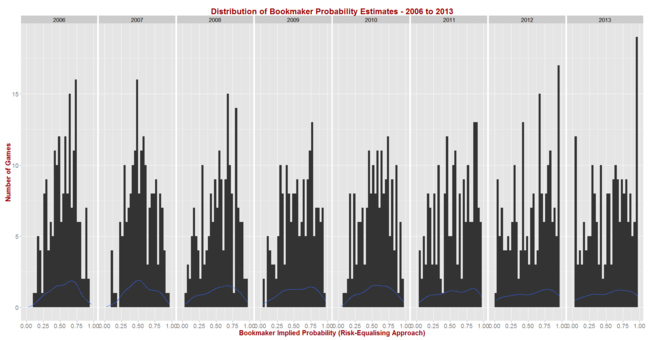
The black bars reflect the number of games for which the home team's implicit home team probability fell into the bin-range recorded in the x-axis, and the blue lines map out the smoothed probability density of that same data. These blue lines highlight the similarity in terms of the profile of home team probabilities of the last three seasons. In these three years we've seen quite high numbers of short-priced (ie high probability) home team favourites and few - though not as few as in some other years - long-shot home teams.
Seasons 2008, 2009 and 2010 saw a more even spread of home team probabilities and fewer extremes of probability at either end, though home team favourites still comfortably outnumbered home team underdogs. Seasons 2006 and 2007 were different again, with 2006 exhibiting some similarities to the 2008 to 2010 period, but with 2007 standing alone as a season with a much larger proportion of contests pitting relatively evenly-matched tips. That characteristic makes prediction more difficult, which we'd expect to be reflected in expected probability scores.
So, with a view to assessing the typical range of Brier Scores under the most diverse sets of conditions, I ran the simulation steps described above once using the home team probability distribution from 2013, and once using the distribution from 2007.
THE BRIER SCORE RESULTS
Here, firstly, are the results for all (bias, sigma) pairs, each simulated for 1,000 seasons that look like 2013.

As we'd expect, the best average Brier Scores are achieved by a tipster with zero bias and the minimum, 1% standard deviation. Such a tipster could expect to achieve an average Brier Score of about 0.167 in seasons like 2013.
For a given standard deviation, the further is the bias from zero the poorer (higher) the expected Brier Score and, for a given bias, the larger the standard deviation the poorer the expected Brier Score as well. So, for example, we can see from the graph that an unbiased tipster with a 5% point standard deviation should expect to record an average Brier Score of about 0.175.
Using Eureqa to fit an equation to the Brier Score data for all 210 simulated (bias, sigma) pairs produces the following approximation:
Expected Brier Score = 0.168 + 0.89 x Bias^2 + 0.87 x Sigma^2
This equation, which explains 98% of the variability in the average Brier Scores across the 210 combinations, suggests that the Brier Score of a tipster is about equally harmed by equivalent changes in percentage point terms in bias and variance (ie sigma squared). Every 1% point change in squared bias or in variance adds about 0.09 to the expected Brier Score.
Next, we simulate Brier Score outcomes for seasons that look like 2007 and obtain the following picture:
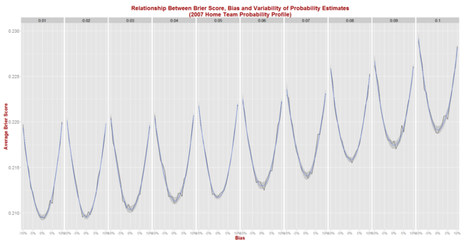
The general shape of the relationships shown here are virtually identical to those we saw when using the 2013 data, but the expected Brier Score values are significantly higher.
Now, an unbiased tipster with a 1% point standard deviation can expect to register a Brier Score of about 0.210 per game (up from 0.167), while one with a 5% point standard deviation can expect to return a Brier Score of about 0.212 (up from 0.175).
Eureqa now offers the following equation to explain the results for the 210 (bias, sigma) pairs:
Expected Brier Score = 0.210 + 0.98 x Bias^2 + 0.94 x Sigma^2
This equation explains 99% of the variability in average Brier Scores across the 210 combinations and, when compared with the earlier equation, suggests that:
- A perfect tipster - that is one with zero bias and zero variance - would achieve a Brier Score of about 0.210 in seasons like 2007 and of 0.168 in seasons like 2013
- Additional bias and variability in a tipster's predictions are punished more in absolute terms in seasons like 2007 than in seasons like 2013. This is evidenced by the larger coefficients on the bias and variance terms in the equation for 2007 compared to those for 2013.
In seasons in which probability estimation is harder - that is, in seasons full of contests pitting evenly-matched teams against one another - Brier Scores will tend to do a better job of differentiating weak from strong predictors.
THE LPS RESULTS
Though I have performed simulations to determine empirical norms for the LPS metric before, I included this metric in the current round of simulations as well. Electrons are cheap.
Here are the curves for simulations of LPS for the 2013-like seasons.
Eureqa suggests that the relationship between expected LPS, bias and variance is, like that between Brier Score, bias and variance, quadratic in nature, though here the curves are concave rather than convex. We get:
Expected LPS = 0.271 - 4.68 x Bias^2 - 4.71 x Sigma^2
This equation explains 99% of the variability in average LPSs observed across the 210 combinations of bias and sigma.
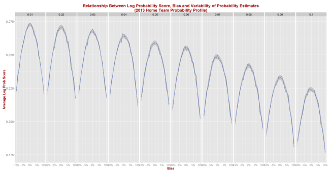
Finally, simulating using 2007-like seasons gives us this picture.

Again we find that the shape when using the 2007 data is the same as that when using the 2013 data, but the absolute scores are poorer (which here means lower).
Eureqa now offers up this equation:
Expected LPS = 0.127 - 4.17 x Bias^2 - 4.35 x Sigma^2
This equation accounts for 97% of the total variability in average LPS across the 210 simulated pairs of bias and sigma and suggests that expected LPSs in seasons like 2007 are less sensitive to changes in bias and variance than are expected LPSs in seasons like 2013. This is contrary to the result we found for expected Brier Scores, which were more sensitive to changes in bias and variance in seasons like 2007 than in seasons like 2013.
In more challenging predictive environments, therefore, differences in predictive ability as measured by different biases and variances, are likely to result in larger absolute differences in Brier Scores than differences in LPSs.
SUMMARY AND CONCLUSION
We now have some bases on which to make normative judgements about Brier Scores and Log Probability Scores, though these judgements require some knowledge about the underlying distribution of true home team probabilities.
If 2014 is similar to the three seasons that have preceded it then a "good" probability predictor should produce an average Brier Score of about 0.170 to 0.175, and an average LPS of about 0.230 to 0.260. In 2013, the three bookmaker-derived Probability Predictors all finished the season with average LPS' of about 0.260.
[EDIT : It's actually not difficult to derive the following relationship theoretically for a forecaster whose predictions are 0 or 1 with fixed probability and independent of the actual outcome
Expected Brier Score = True Home Probability x (1 - True Home Probability) + Bias^2 + Sigma^2
The proof appears in the image at left.
(Click on the image for a larger version.)
Now the fitted equations for Expected Brier Scores above have coefficients on Bias and Sigma that are less than 1 mostly due, I think, to the effects of probability truncation, which tend to improve (ie lower) Brier Scores for extreme probabilities. There might also be some contribution from the fact that I've modelled the forecasts using a Normal rather than a Binomial distribution.
Deriving a similar equation theoretically rather than empirically for the Expected LPS of a contest is a far more complicated endeavour ...]
Is That A Good Probability Score?
/Each week over on the Wagers & Tips blog, and occasionally here in the Statistical Analysis blog I use probability score as a measure of a probability predictor's performance.
Read MoreSimulating SuperMargin Wagering
/Season 2013 has been a good one, so far, for SuperMargin wagering, which led me to ponder why that might be the case. More generally, I wondered if we could define the characteristics of a season and of the predictive algorithm that we're using for selecting wagers, which are most propitious for this form of wagering.
Read MoreAnd the Last Shall be First (At Least Occasionally)
/So far we've learned that handicap-adjusted margins appear to be normally distributed with a mean of zero and a standard deviation of 37.7 points. That means that the unadjusted margin - from the favourite's viewpoint - will be normally distributed with a mean equal to minus the handicap and a standard deviation of 37.7 points. So, if we want to simulate the result of a single game we can generate a random Normal deviate (surely a statistical contradiction in terms) with this mean and standard deviation.
Alternatively, we can, if we want, work from the head-to-head prices if we're willing to assume that the overround attached to each team's price is the same. If we assume that, then the home team's probability of victory is the head-to-head price of the underdog divided by the sum of the favourite's head-to-head price and the underdog's head-to-head price.
So, for example, if the market was Carlton $3.00 / Geelong $1.36, then Carlton's probability of victory is 1.36 / (3.00 + 1.36) or about 31%. More generally let's call the probability we're considering P%.
Working backwards then we can ask: what value of x for a Normal distribution with mean 0 and standard deviation 37.7 puts P% of the distribution on the left? This value will be the appropriate handicap for this game.
Again an example might help, so let's return to the Carlton v Geelong game from earlier and ask what value of x for a Normal distribution with mean 0 and standard deviation 37.7 puts 31% of the distribution on the left? The answer is -18.5. This is the negative of the handicap that Carlton should receive, so Carlton should receive 18.5 points start. Put another way, the head-to-head prices imply that Geelong is expected to win by about 18.5 points.
With this result alone we can draw some fairly startling conclusions.
In a game with prices as per the Carlton v Geelong example above, we know that 69% of the time this match should result in a Geelong victory. But, given our empirically-based assumption about the inherent variability of a football contest, we also know that Carlton, as well as winning 31% of the time, will win by 6 goals or more about 1 time in 14, and will win by 10 goals or more a litle less than 1 time in 50. All of which is ordained to be exactly what we should expect when the underlying stochastic framework is that Geelong's victory margin should follow a Normal distribution with a mean of 18.8 points and a standard deviation of 37.7 points.
So, given only the head-to-head prices for each team, we could readily simulate the outcome of the same game as many times as we like and marvel at the frequency with which apparently extreme results occur. All this is largely because 37.7 points is a sizeable standard deviation.
Well if simulating one game is fun, imagine the joy there is to be had in simulating a whole season. And, following this logic, if simulating a season brings such bounteous enjoyment, simulating say 10,000 seasons must surely produce something close to ecstasy.
I'll let you be the judge of that.
Anyway, using the Wednesday noon (or nearest available) head-to-head TAB Sportsbet prices for each of Rounds 1 to 20, I've calculated the relevant team probabilities for each game using the method described above and then, in turn, used these probabilities to simulate the outcome of each game after first converting these probabilities into expected margins of victory.
(I could, of course, have just used the line betting handicaps but these are posted for some games on days other than Wednesday and I thought it'd be neater to use data that was all from the one day of the week. I'd also need to make an adjustment for those games where the start was 6.5 points as these are handled differently by TAB Sportsbet. In practice it probably wouldn't have made much difference.)
Next, armed with a simulation of the outcome of every game for the season, I've formed the competition ladder that these simulated results would have produced. Since my simulations are of the margins of victory and not of the actual game scores, I've needed to use points differential - that is, total points scored in all games less total points conceded - to separate teams with the same number of wins. As I've shown previously, this is almost always a distinction without a difference.
Lastly, I've repeated all this 10,000 times to generate a distribution of the ladder positions that might have eventuated for each team across an imaginary 10,000 seasons, each played under the same set of game probabilities, a summary of which I've depicted below. As you're reviewing these results keep in mind that every ladder has been produced using the same implicit probabilities derived from actual TAB Sportsbet prices for each game and so, in a sense, every ladder is completely consistent with what TAB Sportsbet 'expected'.

The variability you're seeing in teams' final ladder positions is not due to my assuming, say, that Melbourne were a strong team in one season's simulation, an average team in another simulation, and a very weak team in another. Instead, it's because even weak teams occasionally get repeatedly lucky and finish much higher up the ladder than they might reasonably expect to. You know, the glorious uncertainty of sport and all that.
Consider the row for Geelong. It tells us that, based on the average ladder position across the 10,000 simulations, Geelong ranks 1st, based on its average ladder position of 1.5. The barchart in the 3rd column shows the aggregated results for all 10,000 simulations, the leftmost bar showing how often Geelong finished 1st, the next bar how often they finished 2nd, and so on.
The column headed 1st tells us in what proportion of the simulations the relevant team finished 1st, which, for Geelong, was 68%. In the next three columns we find how often the team finished in the Top 4, the Top 8, or Last. Finally we have the team's current ladder position and then, in the column headed Diff, a comparison of the each teams' current ladder position with its ranking based on the average ladder position from the 10,000 simulations. This column provides a crude measure of how well or how poorly teams have fared relative to TAB Sportsbet's expectations, as reflected in their head-to-head prices.
Here are a few things that I find interesting about these results:
- St Kilda miss the Top 4 about 1 season in 7.
- Nine teams - Collingwood, the Dogs, Carlton, Adelaide, Brisbane, Essendon, Port Adelaide, Sydney and Hawthorn - all finish at least once in every position on the ladder. The Bulldogs, for example, top the ladder about 1 season in 25, miss the Top 8 about 1 season in 11, and finish 16th a little less often than 1 season in 1,650. Sydney, meanwhile, top the ladder about 1 season in 2,000, finish in the Top 4 about 1 season in 25, and finish last about 1 season in 46.
- The ten most-highly ranked teams from the simulations all finished in 1st place at least once. Five of them did so about 1 season in 50 or more often than this.
- Every team from ladder position 3 to 16 could, instead, have been in the Spoon position at this point in the season. Six of those teams had better than about a 1 in 20 chance of being there.
- Every team - even Melbourne - made the Top 8 in at least 1 simulated season in 200. Indeed, every team except Melbourne made it into the Top 8 about 1 season in 12 or more often.
- Hawthorn have either been significantly overestimated by the TAB Sportsbet bookie or deucedly unlucky, depending on your viewpoint. They are 5 spots lower on the ladder than the simulations suggest that should expect to be.
- In contrast, Adelaide, Essendon and West Coast are each 3 spots higher on the ladder than the simulations suggest they should be.
(In another blog I've used the same simulation methodology to simulate the last two rounds of the season and project where each team is likely to finish.)