In-Game Momentum : Score-by-Score Analysis
/So far, in the quest to find evidence for momentum in various guises, I've looked at:
- Something that I called "game cadence" in a post back in 2009 in which I found evidence that the team that won one quarter was less likely to win the next quarter if we considered the entire history of VFL/AFL but more likely to win the next quarter if we narrowed our focus to the period from 1980 onwards. Note that this analysis does not attempt to account for differences in team strength.
- The win-loss progression for each team in another post, this one from 2010 in which I found that many teams were more likely to win a game having won their previous game than their long-term winning rate would suggest and that, similarly, many teams were more likely to lose a game having lost at their previous outing than their long-term losing rate would suggest. This analysis spanned 10 seasons, so it's conceivable that teams' base winning rates might have changed during that period. As such, some of the apparent momentum in successive team results might be attributed to such changes in underlying ability rather than to the short-term effects of the previous week's result. (I updated and expanded on this analysis a little in a subsequent post.)
- The extent to which the final margin of victory for the Home team can be predicted using, along with its leads at the end of each quarter, the change in these leads across quarters. In this formulation, momentum could be said to exist if the Home team's victory margin depended on the rate of change of its lead, not just its actual lead. I investigated this approach in this post from early 2012, finding that the size of any such momentum effect was small.
- Whether the pattern of team scoring in successive quarters suggested that momentum existed in the sense that a team outscoring its opponent in one quarter was more likely to outscore them again in the next. This angle was explored in a post from late 2012. In an attempt to control for the fact that successive quarters of outscoring might be due to underlying team superiority rather than to short-term momentum effects, I looked only at games where each side had outscored its opponents in at least one quarter of the game. I found some evidence for momentum, especially in the 4th quarter for teams that had been outscored in the 1st quarter but that had then gone on to outscore their opponents in the 2nd and 3rd quarters. But, as I noted there, this might instead be evidence only for the existence of games where the stronger team started slowly and then found its rhythm, rather than for the existence of momentum.
- In this post, also from late 2012, the surprising lumpiness of randomness and how this could easily lead a spectator to conclude that scoring ran in streaks when, in fact, the observed scoring was completely consistent with teams scoring at random based on an underlying, constant probability of being the next scorer.
In-Game Momentum - Who Scores What, Next?
What's been missing so far is an empirical search for momentum at the level of the next team to score in a game. Such an analysis requires access to game scoring sequences - which team scored next, when and whether it was a goal or a behind - no readily accessible source of which I'd discovered until recently when I came across the "Scoring Progression" section on the scorecards for each of the games at afltables site. Here, for example, is the information for the first game of season 2012.
The Data
For this current analysis I manually cut-and-pasted scoring progression data from the site for 100 randomly-selected games from the home-and-away season of 2012.

I used Excel's RAND() function to choose the games to include and, as if to gently or mockingly remind me of the lumpiness of random selections, Excel offered up a sample that included only 1 of Hawthorn's home games, but 8 of Port's home fixtures and 8 more of the Dogs' road trips. Unless you think that games involving particular teams are more or less likely to exhibit momentum then the team composition of the random sample is, however, no more than an ironic curiosity.
Excel treated the 23 rounds of the home-and-away season in a slightly more egalitarian manner, selecting a minimum of 2 and a maximum of 7 games from any single round.
Profiling the sample by day of the week we find 54 Saturday, 31 Sunday, 10 Friday, 2 Thursday, 2 Monday and 1 Wednesday game, which seems about right.
I will at some point revisit the ground I cover in this blog if I find a way to access a larger sample of games more efficiently, but for now the 100 chosen games will suffice.
The statistical metric I'll be employing in this blog in the hunt for signs of momentum is "runs" or sequences. If the sequence of scoring in a game was Sydney - Hawthorn - Hawthorn - Sydney - Sydney, that sequence would be said to contain 3 scoring runs: a run of length 1 for Sydney, followed by a run of length 2 for Hawthorn, and then a run of length 2 for Sydney.
Here's the runs data for an actual game, which might give you a feel for the range of numbers that we're likely to encounter. (Please click on the image to access a larger, readable version of it.) Note that I allow runs to span quarters, so a team that scores last in one quarter and first in the next is assessed as having preserved the streak.
In this game there were 17 scoring runs, 8 for Fremantle and 9 for Richmond, which spanned the game's 46 scoring shots. This, it turns out, is about 5.4 fewer runs than we'd expect, making this a game providing strong evidence for team momentum. (The runs variable has been shown to be asymptotically distributed as a Normal with a mean of (2 x Number of Scoring Shots by Team A x Number of Scoring Shots by Team B) / Total Number of Scoring Shots + 1 and a variance that you can find in the Wikipedia page just linked. Monte Carlo simulation I've performed for realistic scoring shot data shows that the Normal approximation of the mean is very good for the range of values we're likely to encounter.)
Knowing the statistical distribution of the runs statistic allows us to perform standard hypothesis testing of the number of runs observed for each game in the sample, which I'll come to in a moment.
If momentum effects are evident in the scoring sequence of games such that the team that scored last is more likely to score next then we'd expect to find fewer, longer runs of scoring than would be the case if no such momentum existed. That means we want to test if the observed number of runs is in the left-hand tail of the distribution. Alternatively, we might postulate that teams tend to respond to being scored against by lifting their effort and, in so doing, become more likely to score next. This would lead to fewer scoring runs than a random sequence would produce. To test this hypothesis we need to determine if the runs statistic is too far into the right-hand tail of the distribution.
Statistically Testing Whether There's Momentum in the Scoring Progression
Formally, the statistical test I'm using is the exact runs test as implemented in the pruns.exact function in the randomizeBE package of R. It calculates the actual distribution of the runs statistic under the null hypothesis of random scoring rather than relying on the Normal approximation discussed above, but the principle is the same. The test requires three inputs: the number of runs observed and the number of scoring shots registered by each team. In essence what we're asking is the following:
Given that Team A registered X scoring shots during the game and Team B registered Y scoring shots, if those scoring shots were organised at random how likely is it that we would have observed as many or more (or as few or less) as the R runs of scoring shots that we actually observed?
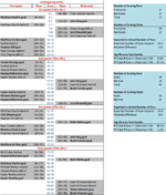
Each of the 100 chosen games has its own values of X, Y and R which can be input into the runs test to calculate the probability that we would have observed a number of runs at least as extreme as we did under the "null hypothesis" that the scoring took place at random (subject to the fixed number of scoring shots for each team). The following table records the p-values so obtained for each of the 100 games.

The numbers on the left relate to the p-values for how likely it was that we would observe a number of runs equal to or less than the number that we actually observed given the null hypothesis of random scoring, and the numbers on the right relate to the p-values for how likely it was that we would observe a number of runs equal to or greater than the number that we actually observed given the null hypothesis of random scoring.
What this table suggests is that, if there is momentum in AFL scoring patterns, it has only a very subtle influence. For starters, we have only 12 games that provide evidence against the null hypothesis at the 10% level, which is only 2 more games than we'd expect to find with p-values in this range due to chance. Even if we look at the number of games delivering a p-value under 50% we've only an excess of 8 games relative to chance.
In one, quite technical way, the runs test makes it hard to detect momentum because the observed number of runs is a discrete rather than a continuous statistic and therefore carries non-zero probability. (I expect that this would be less of an issue if we had a larger sample, but that's to be determined on another day.) One practical consequence of this is a complication in determining statistical significance. If, for example, under the null hypothesis, only 3% of runs values are less than the value we observed, but 88% are greater - because the exact number of runs we observed has a 9% probability under the null hypothesis - is this result statistically significant at the 10% level or not? The p-value for such a game is 12% and so would be recorded in the table above in the 10-20% bucket. Generally, the discrete characteristic of the runs statistic will tend to push the p-values into higher buckets.
Putting that to one side for a moment, there is a formal test that we can use on the set of p-values that we've observed to ask if they, as a group, support or impugn the null hypothesis. It's the Fisher Test, which is described here, and which uses the statistic -2 x sum of the natural logs of the p-values that is distributed under the null hypothesis as a chi-squared variable with 2k degrees of freedom where the number of independent p-values you have is k. In our case, for the p-values on the left-hand side of the table, the statistic is 211.9, which itself has a p-value of 27%. Not even the most null-hypothesis loathing researcher uses an alpha of 30% for his or her hypothesis testing.
We can rescue the possibility of scoring momentum somewhat by looking instead at the proportion of p-values that are less than 50%, treating this statistic as the outcome of a binomial process with constant probability 0.5, and determining whether we have a statistically significantly under- or over-representation of such p-values noting that, under the null hypothesis, we'd expect half of the p-values to be under 50% and half over 50%. With 58 of the 100 observed p-values coming in under 50% we get a p-value for this binomial test of 7%.
Finally, we can lend another sliver of support to the idea of momentum - in a slightly roundabout manner - by performing similar calculations with the p-values from the righthand side of the table above, which are p-values where the alternative hypothesis is that we've witnessed too many runs. The Fisher statistic for these data yield a p-value of 100% and the binomial on the number of p-values less than 50% is 99.9%, both of which are so supportive of the null hypothesis as to imply that we've maybe "chosen the wrong tail" to look at. We should note, however, that the same effect which tends to push the p-values higher for the left-tail test also pushes the p-values higher for the right-tail test, because in both cases we're including the probability associated with the actual observed number of runs in the p-value.
The Verdict on Scoring Momentum for Teams
In short, the evidence is that team scoring streaks are about what we'd expect them to be if momentum did not exist, though there might be some traces of momentum in a handful of games.
Perhaps the best way to put all of this complex statistical analysis in perspective is to look at the effect size of the phenomenon we're dealing with here and to note that the average difference across the 100 games in the sample between the observed and the expected number of runs under the null hypothesis is just 0.7 runs per game. When you consider that the average game has just over 24 scoring runs, that's a tiny if-at-all-existent difference.
What About Momentum in Scoring Type?
We can also ask of the scoring progression data whether or not there's evidence that goals tend to be followed by goals and behinds by behinds, regardless of which team scores them, or whether, instead, there's evidence that goals beget behinds and behinds beget goals - or whether there's no pattern at all to the sequence of scoring.
The following table was created in the same way as the previous table except this time, rather than looking at whether the Home or the Away team scored, we look at whether the score was a goal or a behind, regardless of which team scored it.

Adopting the same approach as we did with the earlier analysis we find that:
- for the distribution of p-values on the left, which has as the alternative hypothesis that we've seen too few scoring streaks to be consistent with the null hypothesis of random scoring, the Fisher statistic has a p-value of 99% and the binomial a p-value of 97%.
- for the distribution of p-values on the right, which has as the alternative hypothesis whether we've seen too many scoring streaks, the Fisher statistic has a p-value of 37% and the binomial a p-value of 31%.
The Verdict on Scoring Momentum by Score Type
Once again the results are inconclusive and lend only very weak, if any, support to the hypothesis that scoring is a fraction too streaky - that is, that goals tend to be followed by behinds, and behinds by goals, rather than goals begetting goals and behinds more behinds.
But here too the effect size is telling. The average difference is the observed number of scoring streaks is -0.5 streaks per game, set against an average number of scoring streaks in a game of 26.1. If there is an effect, it's far too small to notice and far too small to matter.