Modelling Empirical Home Team Victory Probabilities
/In the two blogs so far on the topic of simulating the contest between bookmaker and punter I've not addressed one important aspect of the simulations and that is how to come up with the Home team probabilities for each simulated game.
One, naive approach would be to choose the Home team probability uniformly at random across the interval (0,1), implicitly assuming that a Home team probability of 10% was as likely as a Home team probability of 50%. Empirically these two probabilities are not equally likely; to realistically model a season of AFL wagering we need to model the empirical distribution of Home team probabilities.
A brute-force approach to the problem would have been to build an empirical density function based on historical Home team probabilities and then sample directly from that. So, if a Home Team probability of 25% had occurred in 5% of games, then we'd arrange to select that Home team probability 5% of the time, and do likewise for all other observed Home team probabilities. This would be a practical, if slightly inelegant, solution.
What I instead decided to do was the following:
- Calculate the implicit Home team probability for every game from 1999 to the present.
- Use this to construct an empirical cumulative density function (from which, for example, we could read that, in about 20% of games the Home team's victory probability has been 38% of less).
- Use Eureqa to fit an equation to the empirical cumulative density function
The fitted equation could then be used in the simulations by generating a random variable uniform on the interval (0,1) and then using inputting this value into the equation. This approach ensures that the distribution of Home team probabilities across the simulated seasons roughly approximates the distribution that we've seen over the period from 1999 to now.
So, how well can we fit the empirical distribution of Home team probabilities with a relatively simple equation?
I think it's fair to say that the approach works well, based on this diagram showing the actual and the fitted results:
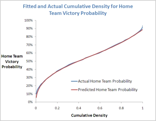
There are some small discrepancies at the extreme values of Home Team Victory Probability, but across the range of Probabilities, the fit is excellent. One of the challenges was to decide the number of points at which to calculate the empirical cumulative density function, and how to space them. Eventually I chose 40 points starting with 10%, 15%, and 20%, and then incrementing in 2% steps to 94% to ensure that I covered the entirety of observed Home team probabilities. This gave me a reasonably smooth curve and seemed to represent the underlying distribution quite well.
The fitted equation is:
Predicted Home Team Probability (for given Cumulative Density) = 0.725 x Cumulative Density^0.408 + 0.165 x Cumulative Density^4
A few facts about the empirical distribution of Home team probabilities since 1999:
- Only a handful of Home teams have been assessed by the bookmaker as having a 10% or lesser chance of victory (just 4 teams in over 2,000 games)
- Only about 1-in-14 Home teams have been assessed as having a 25% or lesser chance of victory
- Only 4-in-10 Home teams have been underdogs or equal favourites
- About 1-in-6 Home teams have been assessed as having a greater than 75% chance of victory
- About 1-in-100 Home teams have been assessed as having a greater than 90% chance of victory
