Bookie v Punter Simulations: An Introduction

For this series of blogs I've built a simulation of a very different kind. It's not designed to simulate team v team but, instead, is about simulating bookie v punter.

To construct these simulations I've assumed that the result of each game is a random binary variable where the true probability of the Home team winning is some constant but unknown True_Home_Prob, the value of which lies between 0 and 1. (For these simulations there are no draws.)

The bookie I'm simulating has the following characteristics, which are held constant for each entire season of wagering:

• His assessment (the usual sexist assumption about the bookmaker applies) of the Home team's probability of victory for a given game, Bookie_Home_Prob, is a random variable with a Normal distribution that has a mean equal to the True_Home_Prob plus a Bookie_Home_Bias (which can be positive, negative or zero) and a fixed standard deviation.
• If the chosen probability for the Home team lands outside the range 0.01 to 0.99 it is reset to whichever of these extremes is closest.
• His overround is a constant 106%.
• The Home team price is set to be the maximum of $1.01 and 1/(Bookie_Home_Prob * Overround)
• The Away team price is set to whatever it needs to be to ensure that 1/Home_Team_Price + 1/Away_Team_Price = Overround

The simulated punter is also assumed to assign a Home team probability that is Normally distributed with a mean equal to the Home_Team_Prob plus a Punter_Home_Bias (which can also be positive, negative or zero) and a fixed standard deviation.

Each replication of the simulation involves 1,000 seasons of 185 games where the respective biases and standard deviations are held fixed across all 1,000 seasons. The Home_Team_Prob for each game is drawn from a distribution that mirrors the distribution of implicit Home team probabilities across the period 1999-2011. (More on this, perhaps, in a future blog.)

Across the entire range of simulations, 6 different types of bookmaker, each described by a pair of values for bias and standard deviation, will be pitted against 10 different types of punter, similarly defined by the two parameters. As well, we'll consider what happens when the punter level-stakes versus Kelly-stakes each game.

In the first simulation a perfect bookmaker, who has 0 bias and 0 standard deviation, is pitted against an unbiased punter with a 2.5% standard deviation in his or her - let's make it a her for balance - assessments of the Home team probability. Practically, that means that about two-thirds of the time she'll be within 5% (ie 2 standard deviations) of the true probability.

Averaged across the 1,000 simulated seasons this matchup sees the punter wager in just over one-quarter of the contests and posting an ROI of around -5% regardless of whether she uses level-staking or Kelly-staking. She can expect to spin a profit in about 40% of seasons played under these assumptions about her and the bookie's characteristics, and the standard deviation of her profit outcome will be quite high, a consequence of the relatively small number of wagers she makes.

The next simulation changes only the standard deviation of the punter's Home team probability assessments, doubling it to 5%. This is not good for her financial prospects and sees her now posting average ROIs of around -6%. She now bets about twice as often, which lowers the standard deviation of her returns, and can expect black ink in only about 30% of seasons.

As we further increase the standard deviation of the punter's Home team probability assessments - to 10% and then 25% - we have little effect on the ROI but we do increase the level of activity, reduce the standard deviation of the returns and slightly lower the likelihood of a profitable season.

Here's the table showing the results of all the simulations (which you can click on for a much larger version):

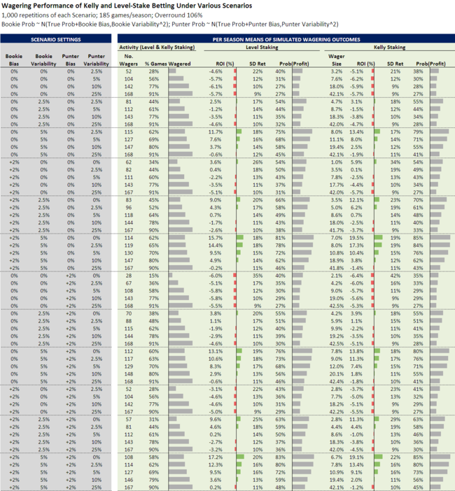
In the second block of simulations we set askew the bookie's halo just a tad by introducing some variability to his Home team probability assessments - just 2.5% for these simulations.

This sliver of vulnerability can be exploited for profit and, interestingly, can be so exploited by a punter with the same characteristics as his. Here for the first time we see the benefit of the punter's ability to abstain from punting when her assessment - rightly or wrongly - suggests it's unwise to do so. In the simulations, a punter with a standard deviation of 2.5% bets in over 40% of contests and generates an ROI of around 2.5-3% depending on staking strategy. She can expect to be profitable in over half of the seasons in which she competes under these conditions.

As we lift the punter's standard deviation, however, we initially snuff out and then proceed to thoroughly demolish the profit opportunity

By the time we reach the third block we're facing a bookie who's likely to be on the cusp of a career change, who has a standard deviation of a whopping (for him) 5%. A punter with a standard deviation as high as 10% is still more likely than not to profit from a season's tussling with such a bookie. If her standard deviation is less than or equal to the bookie's, she'd marginally prefer to be Kelly-staking against him. At a 10% standard deviation, she'd rather be level-staking, though Kelly-staking is nonetheless profitable too.

In the fourth block we introduce a bookie with a small Home-team bias. This makes him very exploitable by a mythical perfect punter - with no bias and zero standard deviation - but also mildly exploitable by one with a 2.5% standard deviation.

Later blocks add variability to the bookie's bias, then bias to the punter, and then both variability and bias to the bookie and to the punter. I'll leave these to the committed reader to review and interpret.

Looking across the 56 combinations that appear in the table, some principles and interesting observations emerge: 

• More variability is always bad for the punter in that it lowers the expected ROI and the probability of making a profit from level- and from Kelly-staking. It also increases the average wager size for Kelly-staking and increase the average number of wagers both for level-staking and for Kelly-wagering.
• A Home team bias for the punter has neither a universally good or bad effect on her returns. This is counterintuitive to me, and needs further investigation.
• A bookie with a zero standard deviation to his Home team probability estimates is very tough to beat unless the punter also has zero standard deviation or the bookie has a mild Home team bias.
• A bookie with non-zero standard deviation is exploitable, even by a punter with a large standard deviation
• Even in the most unfavourable of circumstances - say, for example, a biased punter with a huge standard deviation facing a perfect bookie - a profitable season is only odds of about 3/1.

There's a lot we can do now that this simulation tool is built, for example by modelling the bias and standard deviation as a function of the Home team probability. We can also, using other tools, seek to determine the relative impact of changing the various parameters for the bookie and for the punter on the punter's ROI.