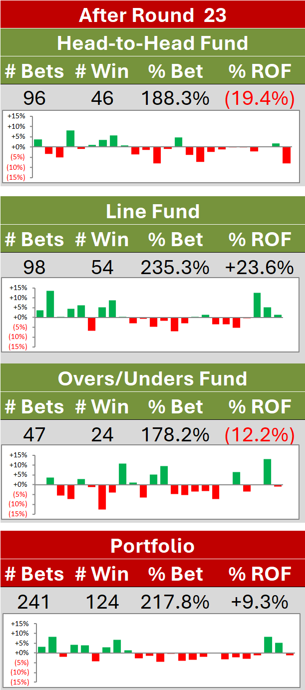
Injecting Variability into Season Projections: How Much is Too Much?
/I've been projecting final ladders during AFL seasons for at least five years now, where I take the current ladder and project the remainder of the season thousands of times to make inferences about which teams might finish where (here, for example, is a projection from last year). During that time, more than once I've wondered about whether the projections have incorporated sufficient variability - whether the results have been overly-optimistic for strong teams and unduly pessimistic for weak teams.
It was for this reason that, last year, I altered the methodology used for projections by incorporating a random perturbation into the team ratings used to simulate each result. Specifically, I added a N(0,0.5) random variable to each team's offensive and defensive MoSSBODS ratings in each game, these alterations feeding directly through into the expected Scoring Shot production of the competing teams. These perturbations serve to increase the chances of upset victories, since additional variability generally helps weaker teams.
(I'm not a fan of the alternative method of introducing greater intra-season randomness - that is, by adjusting team ratings on the basis of within-simulation results - for reasons that I outlined in the blog post linked earlier. In short, my rationale is that it makes no sense at all to change the rating of a team on the basis of a simulated result that was entirely consistent with its original rating. That's like knowing that you're simulating an unbiased die but changing the probability of rolling a six on the second toss just because one happened to show up on the first.)
The standard deviation of 0.5 was justified (lovely passive construction there) on the basis that it was "approximately equal to the standard deviation of MoSSBODS team component rating changes across the last eight or so home-and-away rounds for seasons from 2000 to 2015".
In today's blog I'll be revisiting this approach to season projections and looking to provide a stronger empirical basis to the size of the rating perturbations, if any, to be used in the projections at different points in a season.
USING MOSHBODS TO PROJECT SEASONS
For the analysis I'll be using the new MoSHBODS Team Rating System to provide the basic inputs into the projections - that is, to provide the teams' relative offensive and defensive strengths and the sizes of any venue effects. These will be used to form an initial set of expected scores for both teams in every contest.
The specific questions I'll be looking for the analysis to answer are:
- What is the optimal level of variability to inject into each teams' ratings (or, here, scores derived from those ratings)?
- Does the optimal amount vary during the course of the season as we, potentially, become more accurate in our assessments of team strength?
- Does the metric we use to measure the quality of the projections make any difference to those optima?
With those objectives in mind, the simulations proceed as follows:
- Run the MoSHBODS System on the entire history of V/AFL, saving the team offensive and defensive ratings after every game, as well as the venue performance values for each team at every venue (that is, our best estimate of how much above or below average their performance is likely to be at a particular venue). We do this only to obtain the results for the 2000 to 2016 period, but after every round.
- Consider projecting the final home-and-away season results for each of the 2000 to 2016 seasons as at Round 1, 4, 8, 12, 16, 20, and the next-to-last round in the relevant season.
- Simulate the remainder of the chosen season from the selected round onwards, 1,000 times, using as inputs for the remainder of that season, the actual team ratings and venue performance values as at the end of the previous round. So, if we're projecting from Round 4 of 2015, we use the real MoSHBODS Ratings and Venue Performance Values as at the end of Round 3 of 2015.
- Calculate metrics comparing the simulated seasons with the actual results.
In Step 3 above we simulate the result of every remaining game in the season by:
- Calculating the expected score for each team as the all-team per game average PLUS their Offensive Rating LESS their opponent's Defensive Rating PLUS half the difference between their own and their opponent's Venue Performance Values. (Note that the all-team per game average score is simply the average score per team per game in the previous season).
- Converting this expected score into an expected number of scoring shots, using the average score per scoring shot of teams in the previous season.
- Adding a random amount to the expected number of Scoring Shots by making two independent draws, one for each team, from a N(0, SD) distribution, with SD chosen from the set {0.001, 1, 3, 5, and 7}. The 0.001 choice effectively serves as a "use the raw ratings" option, since an SD of 0.001 effectively returns the mean (ie 0) on every draw.
- Setting the expected number of Scoring Shots equal to 10 if the random perturbation causes it to fall below 10.
- Using a variation of this team scoring model fitted to the 2000 to 2016 seasons, to simulate the scoring in each game.
There will, therefore be 35 distinct simulations (5 SD values by 7 starting Rounds), each of 1,000 replicates, for each of the 17 seasons. That's almost 600,000 in total.
We'll use the following metrics to compare the efficacy of different SD choices at different points in the season:
- The mean absolute difference between all teams' actual and projected end-of-season winning rates
- The mean absolute difference between all teams' actual and projected end-of-season points for and against
- The mean absolute difference between all teams' end-of-season actual and projected ladder finishes
- The Brier Score of the probabilities attached to each of the teams for Making the Top 8, Making the Top 4, and finishing as Minor Premier. We derive the probability estimates based on each team's ladder finishes across the 1,000 relevant replicates.
- The Log Probability Score of the probabilities attached to each of the teams for Making the Top 8, Making the Top 4, and finishing as Minor Premier, using those same probabilities.
- The average number of actual finalists amongst the teams projected to finish in the Top 8.
For all of these metrics except the Log Probability Score and average number of Finalists, lower is better since we'd like to be nearer to the teams' actual winning rates, nearer to their actual points for and against tallies, nearer to their final ladder positions, and better calibrated in terms of their ladder-finish probabilities.
THE RESULTS
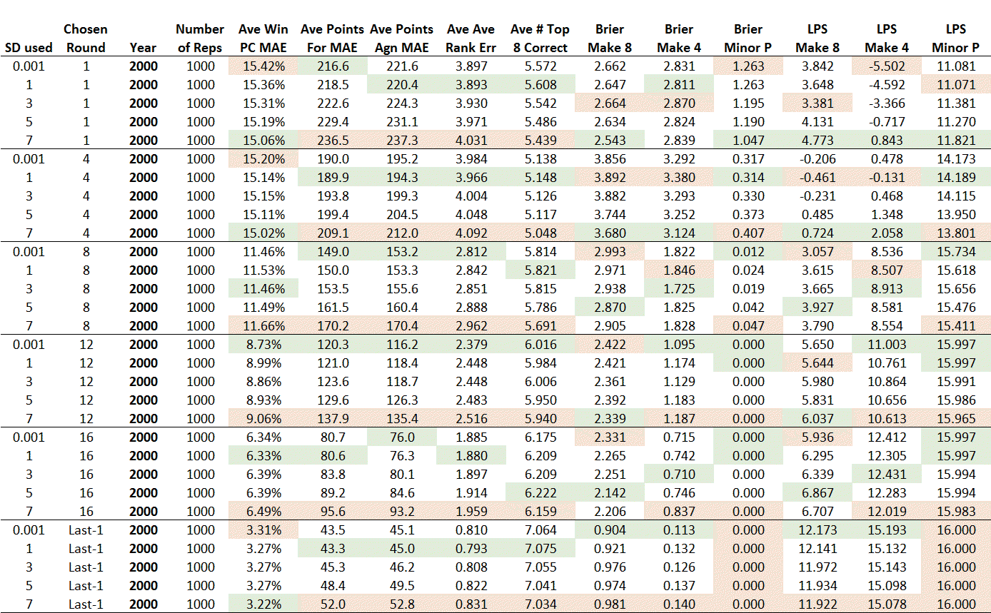
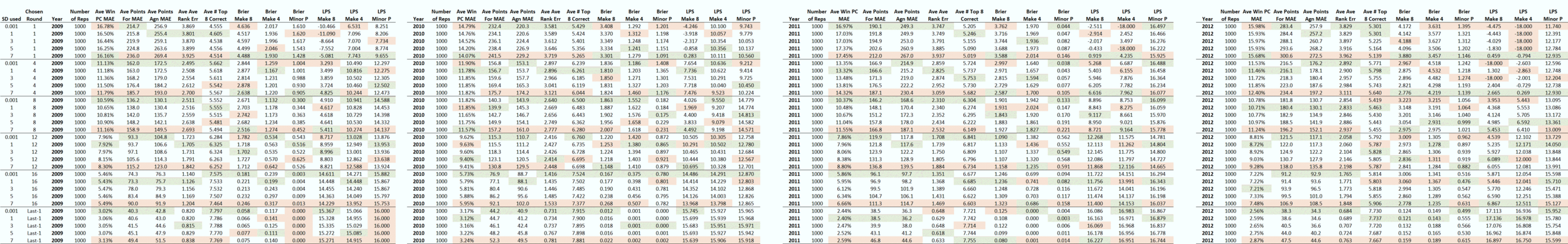
I think the best way of conveying the outputs of the analysis here is as a table.
Let's go through the top five rows.
Each row relates to a different SD being used to perturb team Scoring Shot production, with a given SD used to simulate each season 1,000 times, giving 17,000 replicates in all across the 17 seasons. In this first block, all seasons were simulated from Round 1 to the end of the relevant home-and-away season.
The results were that, on average, teams' :
- projected and actual final winning rates differed in absolute terms by about 15-16% points
- projected and actual points for and against differed, in absolute terms, by about 215-240 points per team
- actual and projected final ladder positions differed, in absolute terms, by about 3.8 to 4.0 places per team (against a naive result of 6 places per team that would be expected in an 18-team competition from someone who ordered the teams at random)
Next, looking at the Brier and Log Probability Scores, we find that:
- the average Brier Score in relation to Top 8 finishes was about 3.4 to 3.6 (against a naive result of 4.2 with an 18-team competition)
- the average Brier Score in relation to Top 4 finishes was about 2.5 to 2.6 (against a naive result of 3.1 with an 18-team competition)
- the average Brier Score in relation to Minor Premiership finishes was about 0.88 to 0.96 (against a naive result of 0.94 with an 18-team competition)
- the average Log Probability Score in relation to Top 8 finishes was between -1.9 and +1.5 (against a naive result of +0.2 with an 18-team competition)
- the average Log Probability Score in relation to Top 4 finishes was between -0.2 and +4.6 (against a naive result of +4.2 with an 18-team competition)
- the average Log Probability Score in relation to Minor Premiership finishes was between 10.3 and 12.1 (against a naive result of +8.9 with an 18-team competition)
Within this block (and every other block) of the table, items shaded in green are the best for a given starting round, while those in red are the worst.
Looking across all the blocks, we see that, within blocks:
- entries relating to an SD of 0.001 are generally best or close to best for the team Win PC, team Points For and team Points Against, team final Rank, and for the average number of Finalists correctly projected to finish in the Top 8.
- entries relating to the largest SD used (7), are generally best for the Brier and Log Probability scores in relation to Top 8 and Top 4 finishes, and in relation to finishing as Minor Premier. The only block where this isn't the case is the very last block, which represents the point in the season where just two rounds remain in the home-and-away season.
In short, there's little convincing evidence to move away from an SD of (effectively) zero at any point in the season if our base assumptions are informed by MoSHBODS and our aim is top predict team winning rates, final scores for and against, final ladder positions, or to select the highest number of Finalists.
Conversely, we'd be better off using quite large SDs if our aim is to calculate the probabilities of teams' finishing in the Top 8 or Top 4, or as Minor Premier.
What this suggests is that the raw ratings do a good job of ordering the teams and simulating the difficulty of their remaining schedules, but also that they provide probabilities that are relatively poorly calibrated.
One way we can improve the calibration of these probabilities is by perturbing the raw Scoring Shot expectations, which tends to move all the probabilities nearer to parity for every team.
Below, for example are the results of 1,000 replicates of the 2016 season, starting in Round 1, using an SD of 0.001 on the left and 7 on the right. You can see that SD = 0.001 provides superior results for all metrics except the Brier and Log Probability Scores.
If you compare the relevant probabilities from which the Scores are calculated, you can see what I mean about them generally being dragged closer to parity when an SD of 7 is used compared to an SD of 0.001. Sydney, for example, were assessed as a 93.4% chance of making the 8 when the SD was 0.001, but only 85.7% chances when the SD was 7. Collingwood, on the other hand, move from 22.8% to 32.5% chances.
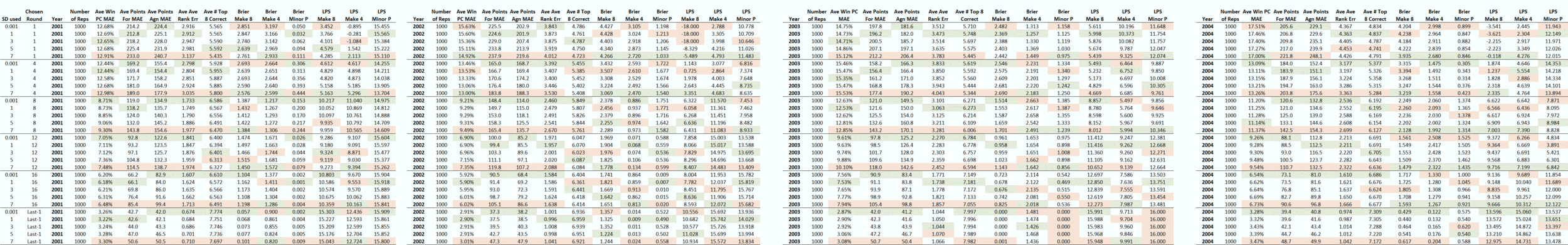
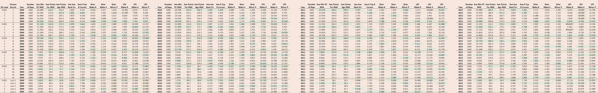
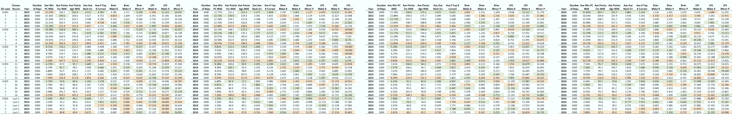
For anyone who's curious, I've provided the season-by-season results below. You'll find that the pattern is fairly consistent and the choice of a zero SD proves best or near-best in most seasons much of the time for all metrics except the probability scores.
(On a technical note, in a few cases, log probability scores were undefined for projections starting at Round 1 or Round 4. This occurs when a team finishes in (say) the Top 8 but the simulations have assigned a probability of zero to that event. In these cases I've arbitrarily recorded a log probability score of -18.)
CONCLUSION
So, what to make of all this?
The most obvious conclusion is that our choice of SD is heavily dependent on the purpose to which we plan to put our season projections. If we're after win percentages, points for and against, ladder finishes of all the teams, or predicting as many finalists as possible, then we should not perturb the raw Scoring Shot expectations at all.
If, instead, we want probability estimates for particular ladder finishes - say top 8, top 4, or minor premier - then we need to perturb the expectations by quite a large amount, possibly by even more than the highest value we've tested here (viz, 7 Scoring Shots). This is a surprising amount of on-the-day variability in Scoring Shot generation. Bear in mind as well that this is in addition to the variability that's already embedded in the team scoring model, both for Scoring Shot production and for conversion rates.
A case could be made, I'd suggest, that probability estimates should be avoided entirely during the earliest parts of the season. Whilst the use of larger SDs for projections commencing in Round 1 do produce probability estimates that are better than those of a naive forecaster (and better than those that use smaller SDs), they are only slightly better.
The case for making probability estimates from about Round 4 is slightly more compelling, but it's not until we get to Round 8 that the gap between optimal projections and naivety becomes very substantial. Another input that would help nudge the scales about when to start making probability estimations would be information about the quality of probability estimates of bookmakers at various points in the season.
I feel as though there's still more quite a bit more to explore in this area - for example, if there's a more elegant and statistically superior way of introducing the extra variability needed - but for today's blog, let's leave it there.