Which Chaser Would You Rather Face?

Many of us have had a lot more time on our hands lately, and I’ve been using some of that watching old episodes of the Australian version of The Chase.

Being of a quantitative mindset, I got to wondering how the prospects of a team’s chances might vary with the Chaser they faced, the target they set for him or her, and the size of the prize fund they’d amassed. So, I Googled around for a dataset and found this amazing Google document from James Spencer via this article of his.

Read More

A Preference For Human Error

Randomness is - as Carl Sagan is oft credited as first declaring - clumpy, and confirmation bias is seductive, so it might be entirely coincidental and partly self-fulfilling that I've lately been noticing common themes in the attitudes towards the statistical models that I create for different people and purposes.

A little context. Some of you will know that as well as building statistical models to predict the outcome of AFL contests as a part-time (sic) hobby, I do similar things during the week, applying those same skills to problems faced by my corporate clients. These clients might, for example, want to identify customers more likely to behave in a specific way - say, to respond to a marketing campaign and open a new product - classify customers as belonging to a particular group or "segment", or talk to customers most at risk of ending their relationship with the client's organisation.

There are parallels between the processes used for modelling AFL results and those used for modelling consumer behaviours, and between the uses to which those models are put. Both involve taking historical data about what we know, summarising the key relationships in that data in the form of a model, and then using that model to make predictions about future behaviours or outcomes.

In football we seek to find relationships between teams' historical on-field performances - who it was that the teams played, where and when, and how they fared - and to generalise those relationships in the form of a model that can be applied to the same or similar teams in future games. With consumers, we take information about who they are, what products and services they use, and how they have used or stopped using those products and services in the past, generalise those relationships via a model, then use that model to predict how the same or similar consumers will behave in the future. 

For both domains that seems a perfectly reasonable approach to take to prediction. Human beings do much the same thing to make their own predictions, albeit intuitively and usually not as systematically or thoroughly. We observe behaviours and outcomes, extract what we think are relevant and causal features of what we observe, generalise that learning and then apply it - sometimes erroneously - to what we perceive to be similar situations in the future. This is how both prejudice and useful generalisations about people and the world are formed. Even intuition, some suggest, is pattern-recognition rendered subconscious.

Now the statistical models we build with data aren't perfect - as George E P Box noted, "... all models are wrong, but some are useful" - but then neither are these heuristic "models" that we craft for ourselves to guide our own actions and reactions. 

Which brings me to my first observation. Simply put, errors made by humans and errors made by statistical models seem to be treated very differently. Conclusions reached by humans using whatever mental model or rule of thumb they employ are afforded much higher status and errors in them, accordingly, forgiven much more quickly and superficially than those reached by a statistical model, regardless of the objective relative empirical efficacy of the two approaches.

This is especially the case if the statistical model is of a type sometimes referred to as a "black box", which are models whose outputs can't be simply expressed in terms of some equation or rule involving the inputs. We humans seem particularly wary of the outputs of such models and impervious to evidence of their objectively superior performance. It's as if we can't appreciate that one cake can taste better than another without knowing all of the ingredients in both.

That's why, I'd suggest, I'll find resolute resistance by some client organisations to using the outputs of a model I've created to select high-probability customers to include in some program, campaign or intervention simply because it's not possible to reverse-engineer why the model identified the customers that it did. Resistance levels will be higher still if the organisation already has an alternative - often unmeasured and untested - rule-of-thumb, historical, always-done-it-that-way-since-someone-decided-it-was-best basis for otherwise selecting customers. There's comfort in the ability to say why a particular customer was included in a program (or excluded from it), which can override any concern about whether greater efficacy might be achieved by choosing a better set of customers using some mysterious, and therefore untrustworthy statistical model.

It can be devastating to a model's perceived credibility - and a coup for the program 'coroner', who'll almost certainly have a personal and professional stake in the outcome - when a few of the apparently "odd" selections don't behave in the manner predicted by the model. If a customer flagged by a model as being a high defection risk turns out to have recently tattooed the company logo on their bicep, another example of boffin madness is quickly added to corporate folklore. 

I find similar skepticism from a smaller audience about my football predictions. No-one thinks that a flesh-and-blood pundit will be capable of unerringly identifying the winners of sporting contests, but the same isn't true for those of us drawing on the expertise of a a statistical model. In essence the attitude from the skeptical few seems to be that, "if you have all that data and all that sophisticated modelling, how can your predictions ever be incorrect, sometimes by quite a lot?" The subtext seems to be that if those predictions are capable of being spectacularly wrong on some occasions, then how can they be trusted at all? "Better to stick with my own opinions however I've arrived at them", seems to be the internal monologue, "... at least I can come up with some plausible post-rationalisations for any errors in them".

But human opinions based on other than a data-based approach are often at least as spectacularly wrong as those from any statistical model, but these too either aren't subjected to close post-hoc scrutiny at all, or are given liberal licence to be explained away via a series of "unforeseeable" in-game events.

Some skeptics are of the more extreme view that there are things in life that are inherently unpredictable using a statistical approach - in the sense of "incapable of being predicted" rather than just "difficult to predict". The outcome of football games is seen by some as being one such phenomenon. 

Still others misunderstand or are generally discomfited by the notion of probabilistic determinism. I can't say with certainty that, say, Geelong will win by exactly 12 points, but I can make probabilistic statements about particular results and the relative likelihood of them, for example claiming that a win by 10 to 20 points is more likely than one by 50 to 60 points.

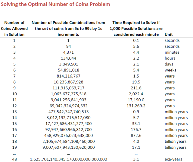
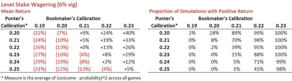
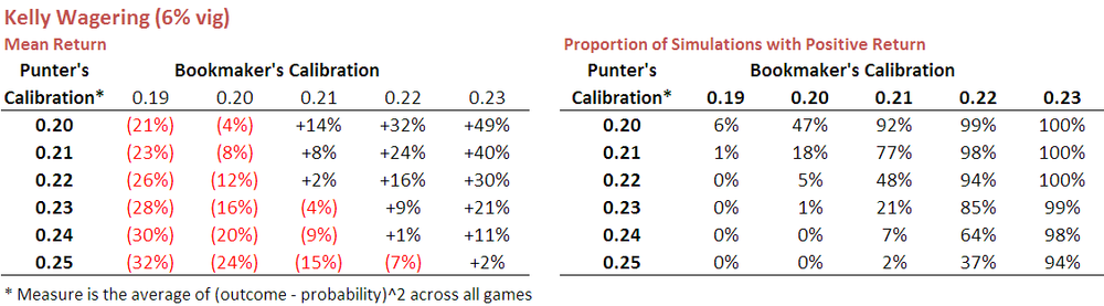
With this view often comes a distrust of the idea that such forecasts are best judged in aggregate, on the basis of a number of such probabilistic assessments of similar events, rather than on an assessment-by-assessment basis. It's impossible to determine how biased or well-calibrated a probabilistic forecaster is from a single forecast, or even from just a few. You need a reasonably sized sample of forecasts to make such an assessment. If I told you that I was able to predict coin tosses and then made a single correct call, I'm sure you wouldn't feel that I'd made my case. But if I did it 20 times in a row you'd be compelled to entertain the notion (or to insist on providing your own coin).

None of this is meant to deride the forecasting abilities of people who make their predictions without building a formal statistical model - in some domains humans can be better forecasters than even the most complex model - but, instead, is an observation that the two approaches to prediction are often not evaluated on the same, objective basis. And, they should be.

WHAT CAN FORECASTERS DO?

As modellers, how might we address this situation then? In broad terms I think we need to more effectively communicate with clients who aren't trained as statistical modellers and reduce the mystery associated with what we do.

With that in mind, here are some suggestions:

1. Better Explain the Modelling Process

In general, we need to better explain the process of model creation and performance measurement to non-technical consumers of our model outputs, and be willing to run well-designed experiments where we compare the performance of our models with those of the internal experts, with a genuine desire to objectively determine which set of predictions are better. 

"Black-box" models are inherently harder to explain - or, at least, their outputs are - but I don't think the solution is to abandon them, especially given that they're often more predictively capable than their more transparent ("white box"?) alternatives. Certainly we should be cautious that our black-box models aren't overfitting history, but we should be doing that anyway.

Usually, if I'm going to build a "black-box" model I'll build a simpler one as well, which allows me to compare and contrast their performance, discuss the model-building process using the simpler model, and then have a discussion to gauge the client's comfort level with the harder-to-explain predictions of the "black-box" model.

(Though the paper is probably a bit too complex for the non-technical client, it's apposite to reference this wonderful Breiman piece on Prediction vs Description here.)

2. Respect and Complement (... and compliment too, if you like) Existing Experts

We need also to be sensitive to the feelings of people whose job has been the company expert in the area. Sometimes, as I've said, human experts are better than statistical models; but often they're not, and there's something uniquely disquieting about discovering your expertise, possibly gleaned over many years, can be trumped by a data scientist with a few lines of computer code and a modicum of data.

In some cases, however, the combined opinion of human and algorithm can be better than the opinion of either, taken alone (the example of Centaur Chess provides a fascinating case study of this). An expert in the field can also prevent a naive modeller from acting on a relationship that appears in the data but which is impractical or inappropriate to act on, or which is purely an artifact of organisational policies or practices. As a real life example of this, a customer defection model I built once found that customers attached to a particular branch were very high defection risks. Time for some urgent remedial action with the branch staff then? No - it turned out that these customers had been assigned to that branch because they had loans that weren't being paid. 

3. Find Ways of Quantitatively Expressing Uncertainty

It's also important to recognise and communicate the inherent randomness faced by all decision-makers, whether they act with or without the help of a statistical model, acknowledging the fundamental difficulties we humans seem to have with the notion of a probabilistic outcome. Football - and consumer behaviour - has a truly random element, sometimes a large one, but that doesn't mean we're unable to say anything useful about it at all, just that we're only able to make probabilistic statements about it.

We might not be able to say with complete certainty that customer A will do this or team X will win by 10 points, but we might be able to claim that customer A is 80% likely to perform some behaviour, or that we're 90% confident the victory margin will be in the 2 to 25 point range. 

Rather than constantly demanding fixed-point predictions - customer A will behave like this and customer B will not, or team X will win by 10 points - we'd do much better to ask for and understand how confident our forecaster is about his or her prediction, expressed, say, in the form of a "confidence interval".

We might then express our 10 point Home team win prediction as follows: "We think the most likely outcome is that the Home team will win by 10 points and we're 60% confident that the final result will lie between a Home team loss by 10 points and a Home team win by 30 points". Similarly, in the consumer example, we might say that we think customer A has a 15% chance of behaving in the way described, while customer B has a 10% chance. So, in fact, the most likely outcome is that neither customer behaves in the predicted way, but if the economics stacks up it makes more sense to talk to customer A than to customer B. Recognise though that there's an 8.5% chance that customer B will perform the behaviour and that customer A will not.

Range forecasts, confidence intervals and other ways of expressing our uncertainty don't make us sound as sure of ourselves as point-forecasts do, but they convey the reality that the outcome is uncertain.

4. Shift the Focus to Outcome rather than Process

Ultimately, the aim of any predictive exercise should be to produce demonstrably better predictions. The efficacy of a model can, to some extent, be demonstrated during the modelling process by the use of a holdout sample, but even that can never be a complete substitute for the in-use assessment of a model.

Ideally, before the modelling process commences - and certainly, before its outputs are used - you should agree with the client on appropriate in-use performance metrics. Sometimes there'll be existing benchmarks for these metrics from similar previous activities, but a more compelling assessment of the model's efficacy can be constructed by supplementing the model's selections with selections based on the extant internal approach, using the organisation's expert opinions or current selection criteria. Over time this comparison might become unnecessary, but initially it can help to quantify and crystallise the benefits of a model-based approach, if there is one, over the status quo.

******

If we do all of this more often, maybe the double standard for evaluating human versus "machine" predictions will begin to fade. I doubt it'll ever disappear entirely though - I like humans better than statistical models too.

Predictive Versus Descriptive Observations

The detailed quantification and numerical dissection of sports started in the US long before it started here in Australia, one result of which has been a modern-day ability to produce statistics so obscure and specific that their half-life is measured in seconds - until the next play, the next pitch, the next batter, the next down, or even just the next statistic. It might well be the case that the Cubs are 7-0 when leading by 3 or more at the Bottom of the 6th when facing a left-handed pitcher at home but what, really, does that tell us about their chances in the current game? Not much, if anything, I'd suggest.

Read More

Who Are The Champions?

Having spent now over seven years applying statistical methods to the analysis and prediction of games of Australian Rules football I've become entirely comfortable - if I was feeling uncharitable I might even say blasé - about treating the outcome of these games as random variables with definable statistical characteristics.
Read More

The Problem With Handling Not Out Scores In Cricket

In cricket, one measure of a batsman's worth is the number of runs the player scores per innings, which is known as the player's average. Calculating this statistic is straightforward for any batsman who's obligingly and unfailingly managed to be dismissed prior to the completion of their team's innings as then it's just a simple division of total runs scored by number of innings batted, but it's problematic as soon as a batsmen has registered a "not out".
Read More

Coins : The Epilogue

Two previous blogs have been devoted to determining the optimal set of coin denominations that would allow one to produce any amount between 5-cents and 95-cents using, on average, the smallest number of coins. So far, we've solved the 2-coin, 3-coin and 4-coin variants of this problem and I flagged, in the most recent blog on the topic, the difficulty I suspected I'd encounter in trying to find solutions for more coins.

A little calculation shows that those concerns were legitimate. The table below shows, for solutions of different sizes - that is, for solutions involving different numbers of coin denominations - how many possible combinations must be considered and how long it would take to consider them using the integer programming routine that I have, which can consider about 1,000 potential solutions per minute.

The curious reader might be interested to know that each combination calculation requires the use of factorials and is of the form 94!/(94-s+1)!(s-1)! where s is the number of coins permitted in the solution. The 94 comes from the fact that there are 94 possible coin denominations to be considered, starting with the 6c and finishing with the 99c. (Note that every potential solution must include a 5-cent piece in order to be capable of producing a solution that delivers a total of 5-cents, and that I've assumed that no optimal solution would include a denomination lower than 5-cents.)

Looking at the final column of the table you can see why I was able to solve the 4-coin problem as it required just a couple of hours of computation, but baulked at attempting the 5-coin problem, which would have needed a couple of days. After that point, things quickly get out of hand.

For example, we'd need a year and a half to topple the 7-coin problem, a generation to solve the 8-coin problem, and a few geological epochs - the exact number depending on which epoch you choose - to address the 15-coiner. The 48-coin solution is the one that would require most time and could be comfortably knocked over in a bit over 3 exa-years - or 3 x 10^18 years if you prefer, which is about 225.6 million times the current best estimate of the age of the universe and, I think, could fairly be labelled 'a while'.

After cracking the 48-coiner it'd all be downhill again, the 49-coin solution taking the same time as the 47-coin solution, the 50-coiner taking the same time as the 46-coiner, and so on.

Facing these sorts of time frames we need, as economists and mathematicians love to say, 'a simplifying assumption'.

In my case what I've decided is to consider as candidate solutions only those involving coins with denominations that are multiples of 5-cents. None of the solutions in the 2-coin, 3-coin or 4-coin problems has involved denominations outside that definition, so I'm taking that as (a somewhat weak) justification of my simplifying assumption.

What this assumption does is turn the 94 in the formula above into an 18, and that makes the identification of solutions feasible during your and my lifetime, which is surely as good an example of the ends justifying the means as any that has ever been posited in the past.

Wielding my freshly-minted assumption as a weapon, I've bludgeoned solutions for the 5-coin through to the 19-coin problems, and the number of solutions for the 5-coin and 6-coin problems are small enough to list here. For the 5-coin problem the solutions are (5,15,25,30,65), (5,15,35,45,50) and (5,20,30,45,55), each of which requires an average of 1.84 coins per transaction, and for the 6-coin problem the solutions are (5,10,25,40,45,50), (5,15,20,25,40,70), (5,15,20,40,45,55), (5,15,20,45,55,80), (5,15,25,30,60,65), (5,15,25,30,65,70) and (5,15,25,35,45,50), each of which requires an average of 1.68 coins per transaction.

The number of solutions for the problems involving more coins rises sharply making these solution lists impractical to provide here. Instead, for completeness, here's a table showing the number of solutions for each sized problem and the average number of coins that this solution requires.

To finish with, here's a graph of how the optimum coins per transaction declines as you allow more and more denominations in the solution.

This graph suggests that there's not much to be gained in going beyond 6 coin denominations, at which point you need, on average, only 1.68 coins per transaction. What's more, if you play with the 6-coin solutions a bit, you'll find that with any of them you'll never need more than 2 coins to complete any transaction from 5-cents to 95-cents, which is something you can't say of any of the 5-coin solutions.

For me then, the optimal optimal solution is (5,15,20,25,40,70). With it, you'll never need more than two coins to produce any total between 5-cents and 95-cents and you should be able to identify the two coins you need quite quickly.

And that, ladies and gentlemen, is the last you'll read here about the coin problem. (Promise.)

We Still Don't Need No 37-cent Piece (And I'm Going Right Off The 10-cent Piece)

A few blogs back we asked and answered the question: if you were to select a set of four coin denominations on the basis that the selected four could combine to make any amount from 5-cents to 95-cents using, on average, the fewest number of them, what would those four denominations be?

There were, it turned out, nine such sets each of which was optimal and required only 2.11 coins, on average, to sum to any amount from 5-cents to 95-cents.

Well since we've solved the problem for 4-coin sets, what about solving it for 2-coin and 3-coin sets?

Only three 2-coin solutions are optimal - (5,20), (5,25) and (5,30) - and each of them requires 3.68 coins on average to produce sums from 5-cents to 95-cents. The combinations of (5,15) and (5,35) are next most efficient, each requiring an average of 4 coins per transaction.

Most efficient amongst what I'd consider to be the odd-looking solutions is (5,12), which requires 7.05 coins per transaction, an average that is bloated by horror outcomes for higher amounts such as the 14 coins required to produce a 95-cent total (5 x 12-cents + 9 x 5-cents).

Moving onto 3-coin solutions we find that there are five that are optimal - (5,15,40), (5,20,30), (5,20,45), (5,25,35) and (5,25,40) - each requiring an average of 2.53 coins per transaction. Glistening amongst the six next-most efficient solutions is (5,20,25), which has the twin virtues of being near-optimal (it requires just 2.63 coins per transaction) and of being patently practical.

Thinking some more about 3-coin solutions, if we were forced to retire one of our current coin denominations, it's the 10-cent that should go as this would leave (5,20,50), a solution that requires an average of only 2.74 coins per transaction. This is only marginally less than optimal in the 3-coin world and is actually not all that much worse than the 2.32 coin average that our current (5,10,20,50) set offers.

Instead of thinking about which of our current coin denominations we might retire, what if, instead, we thought about how we might grow an efficient set of denominations, starting with an optimal set of two coins, then adding a third coin to produce another optimal set, and then finally adding a fourth to again produce an optimal set. Can it be done?

Yes, it can, as is illustrated below.

To produce an all-the-way optimal path from two coins to four we could start with either the (5,20) or the (5,30) sets, though not with the (5,25) set since, although it would allow us to move to an optimal 3-coin solution with the addition of a 35-cent or a 40-cent coin, we would be unable to create an optimal 4-coin solution from there.

For our third coin we could either add the 20-cent coin if we'd started with (5,30), or add the 30-cent or 45-cent coin if we'd started with (5,20).

Lastly, if we'd started with (5,20,45) we could add a 30-cent or a 35-cent coin, or if instead we'd started (5,20,30) we could add a 45-cent or a 65-cent coin to produce an optimal 4-coin solution.

The only way to reach the six other equally optimal 4-coin solutions would have been to start with the sub-optimal (5,15) set, which as we noted earlier falls only a little short of the optimal solutions in requiring on average 4 coins per transaction to the optimal solutions' 3.68 coins per transaction.

I am, naturally, curious about the optimal 5-coin solution (and the 6-coin, and so on) but I don't think that I can find this solution in a practically feasible amount of time using the integer programming optimisation routine that I am currently. Perhaps more at a future date, though probably not.

A Proposition Bet Walks Into a Bar ...

There's time for another quick paradox before the season commences.

Consider the following proposition bet. Each week we'll look at the total points scored in the first game of the round and look at whether the total is even or odd. I win if, across consecutive rounds, the sequence (even,odd,odd) occurs before the sequence (even,odd,even) and you win if the converse occurs. So, for example, if the total scores in the first game of Rounds 1, 2 and 3 were (146, 171, 155) then I'd win. If, instead, they were (132, 175, 162) then you'd win. If no result had been achieved after Round 3 then we'd keep going, starting with the aggregate score for game 1 of Round 4, until one or other of the winning sequences occurred.

Now were I to bet you that my sequence would occur before yours it probably wouldn't surprise you to learn that this is a fair bet at even money odds (recognising that points aggregates for games are as likely to be odd as to be even). But what if, instead, I said that we would play this game repeatedly over the next 3 seasons, with each game ending and another commencing only once both sequences had occurred and that the overall winner of the bet would be the person whose sequence had, on average across all of the completed games, taken the fewest number of games to occur?

So, for example, we might over the course of the three seasons complete 6 games, with my sequence taking 8,6,9,7,11 and 9 games to occur and yours taking 10,11,8,6,10 and 15 games to occur. The average time for my sequence is 50/6 = 8.33 and for your sequence is 60/6 = 10 so, in this case, I'd win.

Given that it's an even money bet whose sequence occurs first would you also be willing to accept even money odds that the average number of games it takes for my sequence to occur will be less than the average number of games it takes for your sequence to occur?

Well if you would, you shouldn't. On average my sequence will take 8 games to occur and yours will take 10 games.

The reason for this apparently paradoxical result is subtle and hinges on how much longer, on average, it takes for the losing sequence to occur after the winning sequence has just been completed. If your sequence - (even,odd,even) - has just occurred then I'm already one-third of the way to completing my sequence of (even,odd,odd), but if my sequence has just occurred then the last result was a game with an odd number of points, so you're still at least three games away from completing your sequence. When you do the maths it turns out that this makes the average number of games required to generate your sequence equal to 10 games while it's only 8 games for my sequence. This despite the fact that it's an even money bet whose sequence turns up first.

You might need to run some simulations with a coin to convince yourself of this, but it is true. A discussion of the result is included in this TED talk from Peter Donnelly. (There are some other fantastic talks on the TED site. While you're visiting you might also want to take a look at the talks by Elizabeth Gilbert, Ken Robinson, Malcolm Gladwell, and a stack of others.)

This result is not, I'll acknowledge, a cracking way to win bar bets - unless, I suppose, you're contemplating a long session, but still expecting to remain sufficiently clear-headed to track a hundred or so coin tosses and to, frankly, give a proverbial about the outcome - but it does have a geeky charm to it.

We Don't Need No 37-cent Piece (But 30- and 45-cent Pieces Might be Nice)

Last night I was reading this Freakonomics blog explaining why a 37-cent piece would make for more efficient US coinage. In the article the question asked was what set of 4 different coin denominations could most efficiently be used to make up any amount between 1c and 99c. Two equally efficient answers were found: a set comprising a 1-cent, 3-cent, 11-cent and 37-cent piece, and one comprising a 1-cent, 3-cent, 11-cent and 38-cent piece. Either combination can be used to produce any total between 1c and 99c using, on average, just 4.1 coins.

Well Australia's different from the US in oh so many ways, and one of those ways is relevant for the present topic: we round all amounts to the nearest 5 cents, having disposed of the 1- and 2-cent pieces in 1991.

So, I wondered, what set of 4 coins would most efficiently meet our needs.

Just so you're clear what I'm on about, consider the 4 coin set comprising a 5 cent, 10 cent, 70 cent and 90 cent piece. A transaction totalling 5 cents can be met with just 1 coin, a transaction of 10 cents can also be met with just one coin, and a transaction of, say, 65 cents can be most efficiently met with 7 coins (1 5-cent piece and 6 10-cent pieces). To determine the overall efficiency of the (5,10,70,90) coin set we calculate how many coins would be needed to meet each transaction size from 5 cents to 95 cents (in 5 cent increments) and we average each of the 19 estimates so obtained. (The answer is 3.16 coins per transaction for this particular combination of denominations, which makes it a fairly inefficient combination, not surprising given that the 70- and 90-cent pieces are useful in so few of the 19 transaction sizes.)

For Australian conditions, it turns out, we'd need to substitute at least two of our current four sub-dollar denominations (viz the 5c, 10c, 20c and 50c pieces) to create an optimal set. Nine solutions are all equally efficient, each requiring an average of about 2.11 coins to meet every amount from 5 cents to 95 cents incrementing in 5 cent lots. The optimal coin sets are:
  • A 5,10,30 and 45 cent solution
  • A 5,15,20 and 45 cent solution
  • A 5,15,35 and 40 cent solution
  • A 5,15,35 and 45 cent solution
  • A 5,15,35 and 60 cent solution
  • A 5,15,40 and 45 cent solution
  • A 5,20,30 and 65 cent solution
  • A 5,20,35 and 45 cent solution
So, Aussies don't need to consider a 37-cent coin, we need to ponder 15-, 35-, 40- and 45-cent coins.

Maybe that's a little too much change (if you'll forgive the dreadful pun). As I noted earlier, each of the optimal solutions listed above necessitates our changing at least two of our existing coin denominations. If you'd prefer that we change only one, the best solution is the (5,10,20,45) set, which is only marginally less efficient than the optimum, requiring an average of 2.21 coins for each transaction in the 5 cent to 95 cent range.

Another sub-optimal but, I contend, attractive option is the (5,10,30,75) set, which needs an average of only 2.16 coins per transaction and which includes a 75-cent piece that would surely come in handy for purchases over a dollar.

Finally, you might be curious how inefficient our current (5,10,20,50) coin set is. It's not too bad, requiring 2.32 coins per transaction, which makes it about 10% less efficient than the optimum.

So the next time you're weighed down with a purse, wallet or pocket full of coins, just think how much more efficient it would be if some of those coins were 30 and 45 cent pieces (and think how much more fun it would be waiting for someone at the checkout to pause, look skyward, give up and then scan a reference sheet to find out how to provide you with the correct change).

A Paradox, Perhaps to Ponder

Today a petite blog on a quirk of the percentages method that's used in AFL to separate teams level on competition points.

Imagine that the first two rounds of the season produced the following results:

Geelong and St Kilda have each won in both rounds and Geelong's percentage is superior to St Kilda's on both occasions (hence the ticks and crosses). So, who will be placed higher on the ladder at the end of the 2nd round?

Commonsense tells us it must be Geelong, but let's do the maths anyway.

  • Geelong's percentage is (150+54)/(115+32) = 138.8
  • St Kilda's percentage is (75+160)/(65+100) = 142.4

How about that - St Kilda will be placed above Geelong on the competition ladder by virtue of a superior overall percentage despite having a poorer percentage in both of the games that make up the total.

This curious result is an example of what's known as Simpson's paradox, a phenomenon that can arise when a weighted average is formed from two or more sets of data and the weights used in combining the data differ significantly for one part compared to the remainder.

In the example I've just provided, St Kilda's overall percentage ends up higher because its weaker 115% in Round 1 is weighted by only about 0.4 and its much stronger 160% in Round 2 is weighted by about 0.6, these weights being the proportions of the total points that St Kilda conceded (165) that were, respectively, conceded in Round 1 (65) and Round 2 (100). Geelong, in contrast, in Round 1 conceded 78% of the total points it conceded across the two games, and conceded only 22% of the total in Round 2. Consequently its poorer Round 1 percentage of 130% carries over three-and-a-half times the weight of its superior Round 2 percentage of 169%. This results in an overall percentage for Geelong of about 0.78 x 130% + 0.22 x 169% or 138.8, which is just under St Kilda's 142.4.

When Simpson's paradox leads to counterintuitive ladder positions it's hard to get too fussed about it, but real-world examples such as those on the Wikipedia page linked to above demonstrate that Simmo can lurk within analyses of far greater import.

(It'd be remiss of me to close without noting - especially for the benefit of followers of the other Aussie ball sports - that Simpson's paradox is unable to affect the competition ladders for sports that use a For and Against differential rather than a ratio because differentials are additive across games. Clearly, maths is not a strong point for the AFL. Why else would you insist on crediting 4 points for a win and 2 points for a draw oblivious, it seems, to the common divisor shared by the numbers 2 and 4?)

Improving Your Tipping

You're out walking on a cold winter's evening, contemplating the weekend's upcoming matches, when you're approached by a behatted, shadowy figure who offers to sell you a couple of statistical models that tip AFL winners. You squint into the gloom and can just discern the outline of a pocket-protector on the man who is now blocking your path, and feel immediately that this is a person whose word you can trust.

He tells you that the models he is offering each use different pieces of data about a particular game and that neither of them use data about which is the home team. He adds - uninformatively you think - that the two models produce statistically independent predictions of the winning team. You ask how accurate the models are that he's selling and he frowns momentarily and then sighs before revealing that one of the models tips at 60% and the other at 64%. They're not that good, he acknowledges, sensing your disappointment, but he needs money to feed his Lotto habit. "Lotto wheels?" , you ask. He nods, eyes downcast. Clearly he hasn't learned much about probability, you realise.

As a regular reader of this blog you already have a model for tipping winners, sophisticated though it is, which involves looking up which team is the home team - real or notional - and then tipping that team. This approach, you know, allows you to tip at about a 65% success rate.

What use to you then is a model - actually two, since he's offering them as a job lot - that can't out-predict your existing model? You tip at 65% and the best model he's offering tips only at 64%.

If you believe him, should you walk away? Or, phrased in more statistical terms, are you better off with a single model that tips at 65% or with three models that make independent predictions and that tip at 65%, 64% and 60% respectively?

By now your olfactory system is probably detecting a rodent and you've guessed that you're better off with the three models, unintuitive though that might seem.

Indeed, were you to use the three models and make your tip on the basis of a simple plurality of their opinions you could expect to lift your predictive accuracy to 68.9%, an increase of almost 4 percentage points. I think that's remarkable.

The pivotal requirement for the improvement is that the three predictions be statistically independent; if that's the case then, given the levels of predictive accuracy I've provided, the combined opinion of the three of them is better than the individual opinion of any one of them.

In fact, you also should have accepted the offer from your Lotto-addicted confrere had the models he'd been offering each only been able to tip at 58% though in that case their combination with your own model would have yielded an overall lift in predictive accuracy of only 0.3%. Very roughly speaking, for every 1% increase in the sum of the predictive accuracies of the two models you're being offered you can expected about a 0.45% increase in the predictive accuracy of the model you can form by combining them with your own home-team based model.

That's not to say that you should accept any two models you're offered that generate independent predictions. If the sum of the predictive accuracies of the two models you're offered is less than 116%, you're better off sticking to your home-team model.

The statistical result that I've described here has obvious implications for building Fund algorithms and, to some extent, has already been exploited by some of the existing Funds. The floating-window based models of HELP, LAMP and HAMP are also loosely inspired by this result, though the predictions of different floating-window models are unlikely to be statistically independent. A floating-window model that is based on the most recent 10 rounds of results, for example, shares much of the data that it uses with the floating-window model that is based on the most recent 15 rounds of results. This statistical dependence significantly reduces the predictive lift that can be achieved by combining such models.

Nonetheless, it's an interesting result I think and more generally highlights the statistical validity of the popular notion that "many heads are better than one", though, as we now know, this is only true if the owners of those heads are truly independent thinkers and if they're each individually reasonably astute.

And May All Your Probabilities Be Well-Calibrated

Say I believe that Melbourne are a 20% chance to win a hypothetical game of football - and some years it seems that this is the only type of game they have any chance of winning - yet you claim they're a 40% chance. How, and when, can we determine whose probability is closer to the truth?

In situations like this one where a subjective probability assessment is required people make their probability assessments using any information they have that they believe is relevant, weighting each piece of that knowledge according to the relative importance they place on it. So the difference between your and my estimates for our hypothetical Melbourne game could stem from differences in the information we each hold about the game, from differences in the relative weights we apply to each piece of information, or from both of these things.

If I know, for example, that Melbourne will have a key player missing this weekend and you don't know this - a situation known as an "information asymmetry" in the literature - then my 20% and your 40% rating might be perfectly logical, albeit that your assessment is based on less knowledge than mine. Alternatively, we might both know about the injured player but you feel that it has a much smaller effect on Melbourne's chances than I do.

So we can certainly explain why our probability assessments might logically be different from one another but this doesn't definitively address the topic of whose assessment is better.

In fact, in any but the most extreme cases of information asymmetry or the patently inappropriate weighting of information, there's no way to determine whose probability is closer to the truth before the game is played.

So, let's say we wait for the outcome of the game and Melbourne are thumped by 12 goals. I might then feel, with some justification, that my probability assessment was better than yours. But we can only learn so much about our relative probability assessment talents by witnessing the outcome of a single game much as you can't claim to be precognitive after correctly calling the toss of a single coin.

To more accurately assess someone's ability to make probability assessments we need to observe the outcomes of a sufficiently large series of events for each of which that person had provided a probability estimate beforehand. One aspect of the probability estimates that we could them measure is how "calibrated" they are.

A person's probability estimates are said to be well-calibrated if, on average and over the longer term, events to which they assign an x% probability occur about x% of the time. A variety of mathematical formulae (see for example) have been proposed to measure this notion.

For this blog I've used as the measure of calibration the average squared difference between the punter's probability estimates and the outcome, where the outcome is either a 1 (for a win for the team whose probability has been estimated) or a 0 (for a loss for that same team). So, for example, if the punter attached probabilities of 0.6 to each of 10 winning teams, the approximate calibration for those 10 games would be (10 x (1-0.6)^2)/10 = 0.16.

I chose this measure of calibration in preference to others because, empirically, it can be used to create models that explain more of the variability in punting returns. But, I'm getting ahead of myself - another figure of speech whose meaning evaporates under the scantest scrutiny.

The table below shows how calibration would be estimated for four different punters.

By way of contexting the calibration score, note that the closer a punter's score is to zero, the better calibrated are his or her probability assessments, and a punter with absolutely no idea, but who knows this and therefore assigns a probability of 0.5 to both team's chances in every game, will have a calibration score of 0.25 (see Punter #2 above). Over the period 2006 to 2009, the TAB Sportsbet bookmaker's probability assessments have a calibration score of about 0.20, so the numerically tiny journey from a calibration score of 0.25 to one of 0.20 traverses the landscape from the township of Wise Ignorance to the city of Wily Knowledge.

Does Calibration Matter?

It's generally desirable to be labelled with a characteristic that is prefixed with the word stem "well-", and "well-calibrated" is undoubtedly one such characteristic. But, is it of any practical significance?

In your standard pick-the-winners tipping competition, calibration is nice, but accuracy is king. Whether you think the team you tip is a 50.1% or a 99.9% chance doesn't matter. If you tip a team and they win you score one; if they lose, you score zero. No benefit accrues from certainty or from doubt.

Calibration is, however, extremely important for wagering success: the more calibrated a gambler's probability assessments, the better will be his or her return because the better will be his or her ability to identify market mispricings. To confirm this I ran hundreds of thousands of simulations in which I varied the level of calibration of the bookmaker and of the punter to see what effect it had on the punter's ROI if the punter followed a level-staking strategy, betting 1 unit on those games for which he or she felt there was a positive expectation to wagering.

(For those of you with a technical bent I started by generating the true probabilities for each of 1,000 games by drawing from a random Normal distribution with a mean of 0.55 and a standard deviation of 0.2, which produces a distribution of home-team and away-team probabilities similar to that implied by the bookie's prices over the period 2006 to 2009.

Bookie probabilities for each game were then generated by assuming that bookie probabilities are drawn from a random Normal with mean equal to the true probability and a standard deviation equal to some value - which fixed for the 1,000 games of a single replicate but which varies from replicate to replicate - chosen to be in the range 0 to 0.1. So, for example, a bookie with a precision of 5% for a given replicate will be within about 10% of the true probability for a game 95% of the time. This approach produces simulations with a range of calibration scores for the bookie from 0.187 to 0.24, which is roughly what we've empirically observed plus and minus about 0.02.

I reset any bookie probabilities that wound up above 0.9 to be 0.9, and any that were below 0.1 to be 0.1. Bookie prices were then determined as the inverse of the probability divided by one plus the vig, which was 6% for all games in all replicates.

The punter's probabilities are determined similarly to the bookie's except that the standard deviation of the Normal distribution is chosen randomly from the range 0 to 0.2. This produced simulated calibration scores for the punter in the range 0.188 to 0.268.

The punter only bets on games for which he or she believes there is a positive expectation.)

Here's a table showing the results.

So, reviewing firstly items from the top row we can say that a punter whose probability estimates are calibrated at 0.20 (ie as well-calibrated as the bookies have been over recent seasons) can expect an ROI of negative 22% if he or she faces a bookie whose probability estimates are calibrated at 0.19. Against a bookie whose estimates are instead calibrated at 0.20, the punter can expect to lose about 7%, or a smidge over the vig. A profit of 9% can be expected if the bookie is calibrated at 0.21.

The table on the right shows just how often the punter can expect to finish in the black - for the row we've been looking at about 2% of the time when facing a bookie calibrated at 0.19, and 89% of the time when facing a bookie calibrated at 0.21.

You can see in these tables how numerically small changes in bookie and punter calibration produce quite substantial changes in expected ROI outcomes.

Scanning the entirety of these tables makes for sobering reading. Against a typical bookie, who'll be calibrated at 0.2, even a well-calibrated punter will rarely make a profit. The situation improves if the punter can find a bookie calibrated at only 0.21, but even then the punter must themselves be calibrated at 0.22 or better before he or she can reasonably expect to make regular profits. Only when the bookie is truly awful does profit become relatively easy to extract, and awful bookies last about as long as a pyromaniac in a fireworks factory.

None of which, I'm guessing, qualifies as news to most punters.

One positive result in the table is that a profit can still sometimes be turned even if the punter is very slightly less well-calibrated than the bookie. I'm not yet sure why this is the case but suspect it has something to do with the fact that the bookie's vig saves the well-calibrated punter from wagering into harmful mispricings more often than it prevents the punter from capitalising on favourable mispricings,

Looking down the columns in the left-hand table provides the data that underscores the importance of calibration. Better calibrated punters (ie those with smaller calibration scores) fare better than punters with poorer calibration - albeit that, in most cases, this simply means that they lose money as a slower rate.

Becoming better calibrated takes time, but there's another way to boost average profitability for most levels of calibration. It's called Kelly betting.

Kelly Betting

The notion of Kelly betting has been around for a while. It's a formulaic way of determining your bet size given the prices on offer and your own probability assessments, and it ensures that you bet larger amounts the greater the disparity between your estimate of a team's chances and the chances implied by the price on offer.

When used in the simulations I ran earlier it produced the results shown in the following table:

If you compare these results with those shown earlier using level-stake wagering you find that Kelly betting is almost always superior, the exception being for those punters with poor calibration scores, that is, generally worse than about 0.24. Kelly betting, it seems, better capitalises on the available opportunities for those punters who are at least moderately well-calibrated.

This year, three of the Fund algorithms will use Kelly betting - New Heritage, Prudence, and Hope - because I'm more confident that they're not poorly-calibrated. I'm less confident about the calibration of the three new Fund algorithms, so they'll all be level-staking this season.

You're Reading This Blog: What An Amazing Coincidence!

While idly surfing the web the other day - and, let's be honest, how often do we surf otherwise - I came across a summary of the most recent 450 Monday Lotto draws (note that the numbers from this site to which I refer in this blog might have changed by the time you view them since they're updated with each draw). For those of you unfamiliar with the NSW Monday Lotto format, 8 balls are chosen at random from 45 numbered balls with the first 6 deemed to comprise the "main" draw and the last two designated "supplementary" balls.

Given that arrangement you'd expect each ball to be drawn amongst the main balls, on average, about every 7 or 8 draws. What caught my eye then was that the ball numbered 30 had gone 37 draws without being vacuumed up as part of the main draw. That's nine months without gulping fresh air, which seemed pretty extraordinary to me. But, the questions is: how extraordinary?

Well, there's a 39 in 45 chance that a particular numbered ball won't be selected in the main draw in any given week, so the chances of that same numbered ball racking up 37 consecutive misses is (39/45)^37 (ie 39/45 raised to the 37th power), which is about 0.5% or, if you prefer, about a 200/1 event. That's a slim chance in anyone's assessment and certainly would be deemed statistically significant in most journal articles. So, do I have grounds for questioning the randomness of the Monday Lotto draw?

Absolutely not. The probability I just calculated applies only to the situation where the long-term unselected ball in question was pre-specified by me, but the situation that actually pertains is that I noticed that ball from amongst the 45 with the longest run of outs. I would have been equally amazed if it had been the ball numbered 5 that had achieved this record, or if it had been the ball numbered 12, or indeed any of the balls. In reality then I had a much greater chance of being amazed.

Just how much greater can readily be estimated via a quick simulation, which I've run and which tells me that I should expect to find at least one number with a run of outs of 37 weeks or longer about 20% of the time. In other words, it's only about a 4/1 shot and hardly worth being amazed about at all. Based on my calculations, we'd need to witness a run of about 47 weeks before we'd raise a statistician's eyebrow, as a run this long is the shortest that would surpass the 5% threshold for statistical significance. Further, we'd need a run of 58 weeks before we'd get that second eyebrow in motion as it'd only be then that we'd have a phenomenon with a probability of being due to chance under 1%.

Of course, events with probabilities even as low as 1% do occur occasionally - Melbourne to finish in the Top 4 anyone - so even if we did observe a run this long we couldn't definitively state that the Lotto draws hadn't been random, though we'd have a much stronger basis on which to suspect this.

My more general point here is how easy it is to be fooled into believing that something we've observed is extraordinary without realising how many non-extraordinary things we observed and discounted before registering the outlier. This psychological bias is the basis for many of the "unbelievable" coincidences credulously reported in the media - the person who wins the lottery for the 2nd time, the family with the Dad and the three kids all born on the same day, and the two holes in one by the same golfer in the same round.

If a lot of stuff's happening, most of it will be ordinary, but some of it must be extraordinary.

Seeking Significance

Distinguishing between a statistical aberration and a meaningful deviation from what's expected is a skill that's decidedly difficult to acquire. If my train to work is late 15 days out of 20 is that a sign that the train is now permanently more likely to be late than to be early?

The TAB offers a 50:50 proposition bet on every AFL game that the match will end with an even or an odd number of points being scored. I can find no reason to favour one of those outcomes over another, so even money odds seems like a reasonable proposition.

How strange it is then that 6 of the last 8 seasons have finished with a preponderance of games producing an even total. Surely this must be compelling evidence of some fundamental change in the sport that's tilting the balance in favour of even-totalled results. Actually, that's probably not the case.

One way to assess the significance of such a run is to realise that we'd have been equally as stunned if the preponderance had been of odd-totalled games and then to ask ourselves the following question: if even-totalled and odd-totalled games were equally likely, over 112 seasons how likely is it that we could find a span of 8 seasons within which there was a preponderance of once type of total over the other in 6 of those seasons?

The answer - which I found by simulating 100,000 sets of 112 seasons - is 99.8%. In other words, it's overwhelmingly likely that a series of 112 seasons should contain somewhere within it at least one such sequence of 6 from 8.

Below is a chart showing the percentage of games finishing with an even total for each if the 112 seasons of the competition. The time period we've just been exploring is that shown in the rightmost red box.

If we go back a little further we can find a period from 1979 to 2000 in which 16 of the 22 seasons finished with a preponderance of seasons with more odd-totalled than even-totalled games. This is the period marked with the middle red box. Surely 16 from 22 is quite rare.

Well, no it isn't. It's rarer than 6 from 8 but, proceeding in a manner similar to how we proceeded earlier we find that there's about a 62% probability of such a run occurring at least once in the span of 112 seasons. So, it's still comfortably more likely than not that we should find such a sequence even if the true probability of an even-totalled game is exactly 50%.

Okay, we've dismissed the significance of 6 from 8 and 16 from 22, but what about the period from 1916 to 1974 (the leftmost red box) during which 37 of the 59 seasons had predominantly odd-totalled games? Granted, it's a little more impressive than either of the shorter sequences, but there's still a 31% chance of finding such a sequence in a 112 season series.

Overall then, despite the appearance of these clusters, it's impossible to reject the hypothesis that the probability of an even-totalled game is and always has been 50%.

Further evidence for this is the fact that the all-time proportion of even-totalled games is 49.6%, a mere 55 games short of parity. Also, the proportion of seasons in which the deviation from 50% is statistically significant at the 1% level is 0.9%, and the proportion of seasons in which the deviation from 50% is statistically significant at the 5% level is 4.5%.

Finding meaningful and apparently significant patterns in what we observe is a skill that's served us well as a species. It's a good thing to recognise the pattern in the fact that 40 of the 42 people who've eaten that 6-day-old yak carcass are no longer part of the tribe.

The challenge is to be aware that this skill can sometimes lead us to marvel at - in some cases even take credit for - patterns that are just statistical variations. If you look out for them you'll see them crop up regularly in the news.